03: Data Structures
Virtual Environments
Section titled “Virtual Environments”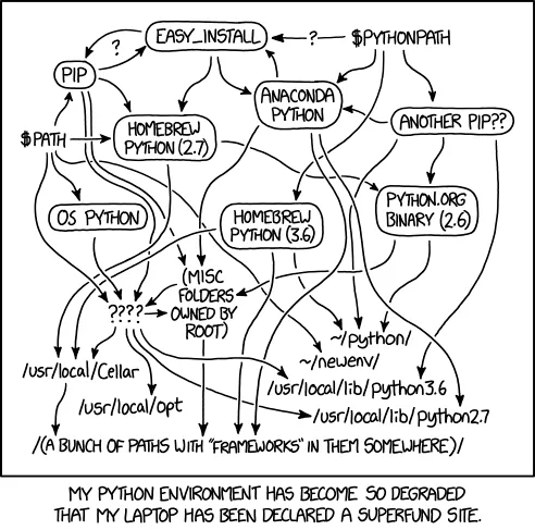
Virtual environments prevent package chaos
Why Virtual Environments?
Section titled “Why Virtual Environments?”The Problem: Different projects need different package versions.
- Project A needs pandas 1.3.0
- Project B needs pandas 2.0.0
- Installing one breaks the other!
The Solution: Each project gets its own Python environment.
Using venv (recommended)
Section titled “Using venv (recommended)”Reference:
# Create environmentpython -m venv datasci-practice
# Activate (Mac/Linux)source datasci-practice/bin/activate
# Activate (Windows)datasci-practice\Scripts\activate
# Install packagespip install pandas numpy matplotlib
# Save requirementspip freeze > requirements.txt
# Deactivatedeactivate
Using uv (Fast & Modern)
Section titled “Using uv (Fast & Modern)”Reference:
# Install uv (if not already installed)curl -LsSf https://astral.sh/uv/install.sh | sh
# Create environmentuv venv datasci-practice
# Activate (Mac/Linux)source datasci-practice/bin/activate
# Activate (Windows)datasci-practice\Scripts\activate
# Install packagesuv pip install pandas numpy matplotlib
# Save requirementsuv pip freeze > requirements.txt
# Deactivatedeactivate
Using Conda
Section titled “Using Conda”Reference:
# Create environmentconda create -n datasci-practice python=3.11
# Activateconda activate datasci-practice
# Install packagesconda install pandas numpy matplotlib
# Deactivateconda deactivate
# Save environmentconda env export > environment.yml
Python Potpourri
Section titled “Python Potpourri”Type Checking
Section titled “Type Checking”Reference:
# Check what type your data isuser_input = "42"print(type(user_input))     # <class 'str'>
number = int(user_input)print(type(number))         # <class 'int'>
F-String Formatting
Section titled “F-String Formatting”Reference:
name = "Alice"grade = 87.5
# F-stringsmessage = f"Student {name} earned {grade:.1f}%"
# Formatting optionsprint(f"Grade: {grade:.2f}")      # 87.50print(f"Grade: {grade:>8.1f}")    # Right-alignedprint(f"Grade: {grade:<8.1f}")    # Left-aligned
# Expressions in f-stringsarr = np.array([1, 2, 3, 4, 5])print(f"Mean: {arr.mean():.2f}")
Why NumPy Matters
Section titled “Why NumPy Matters”Python is famously slow for numerical computing:
# Pure Python approach (SLOW)my_list = list(range(1_000_000))result = [x * 2 for x in my_list]  # 46.4 ms
# NumPy approach (FAST)import numpy as npmy_array = np.arange(1_000_000)result = my_array * 2  # 0.3 ms - 150x faster!
NumPy is 10-100x faster than pure Python for numerical operations.
The NumPy Solution
Section titled “The NumPy Solution”- ndarray: Fast, memory-efficient multidimensional arrays
- Vectorized operations: Apply functions to entire arrays at once
- Broadcasting: Smart handling of different-sized arrays
- Universal functions (ufuncs): Fast element-wise operations
NumPy Quick Reference
Section titled “NumPy Quick Reference”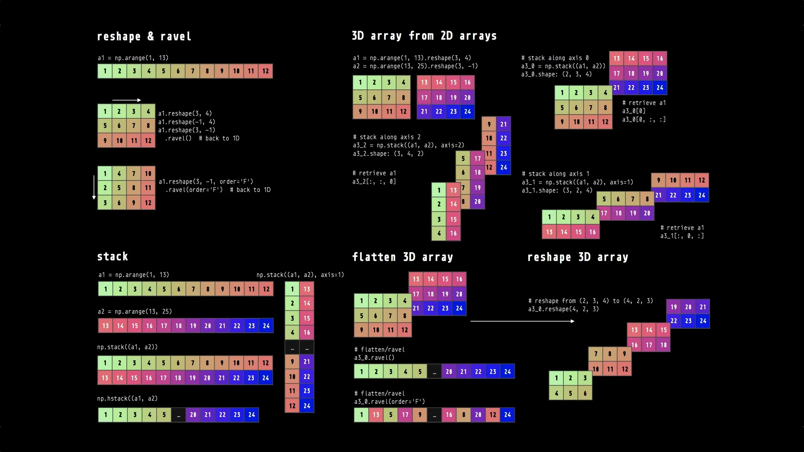
Creating Arrays
Section titled “Creating Arrays”Reference:
import numpy as np
# From Python listsarr = np.array([1, 2, 3, 4, 5])arr_2d = np.array([[1, 2, 3], [4, 5, 6]])
# Array creation functionszeros = np.zeros(5)              # array([0., 0., 0., 0., 0.])ones = np.ones((2, 3))           # 2x3 array of onesrange_arr = np.arange(10)        # array([0, 1, 2, ..., 9])full = np.full((2, 3), 7)        # 2x3 array filled with 7
Array Properties
Section titled “Array Properties”Reference:
arr = np.array([[1, 2, 3], [4, 5, 6]])
print(arr.shape)      # (2, 3) - 2 rows, 3 columnsprint(arr.ndim)       # 2 - number of dimensionsprint(arr.size)       # 6 - total elementsprint(arr.dtype)      # int64 - data type
Data Types
Section titled “Data Types”Reference:
# Explicit data typesarr_int = np.array([1, 2, 3], dtype=np.int32)arr_float = np.array([1, 2, 3], dtype=np.float64)
# Type conversionarr = np.array([1, 2, 3, 4, 5])float_arr = arr.astype(np.float64)
# String to numericstr_arr = np.array(["1.25", "-9.6", "42"])num_arr = str_arr.astype(float)
Array Indexing and Slicing
Section titled “Array Indexing and Slicing”Basic Indexing
Section titled “Basic Indexing”NumPy’s indexing syntax allows you to access and slice array elements using familiar Python notation, extended to work seamlessly across multiple dimensions.
Reference:
arr = np.array([0, 1, 2, 3, 4, 5, 6, 7, 8, 9])
# Single elementfirst = arr[0]          # 0last = arr[-1]          # 9
# Slicingsubset = arr[2:7]       # array([2, 3, 4, 5, 6])every_other = arr[::2]  # array([0, 2, 4, 6, 8])
Multidimensional Indexing
Section titled “Multidimensional Indexing”With multidimensional arrays, you can use comma-separated indices to access elements, rows, or columns, making it easy to work with matrices and higher-dimensional data.
Reference:
arr_2d = np.array([[1, 2, 3], [4, 5, 6], [7, 8, 9]])
# Access elementsfirst_row = arr_2d[0]        # array([1, 2, 3])element = arr_2d[1, 2]       # 6
# Slicingfirst_two_rows = arr_2d[:2]  # First 2 rowsmiddle_column = arr_2d[:, 1] # Column 1: array([2, 5, 8])
Boolean Indexing
Section titled “Boolean Indexing”Boolean indexing allows you to filter arrays using conditional logic, selecting only elements that meet specific criteria. This is essential for data analysis tasks like finding outliers, filtering datasets, or applying conditional transformations.
Reference:
arr = np.array([1, 5, 3, 8, 2, 9, 4])
# Boolean maskmask = arr > 5              # array([False, False, False, True, False, True, False])high_values = arr[mask]     # array([8, 9])
# Conditional operationsarr[arr > 5] = 0            # Set values > 5 to 0
# Multiple conditions (use & for AND, | for OR)mask = (arr > 2) & (arr < 8)filtered = arr[mask]
Fancy Indexing
Section titled “Fancy Indexing”Fancy indexing uses integer arrays to select multiple elements at arbitrary positions in a single operation. This powerful technique enables efficient data reordering, sampling, and custom selection patterns without explicit loops.
Reference:
arr = np.array([10, 20, 30, 40, 50, 60, 70, 80])
# Integer array indexingindices = [1, 3, 5]selected = arr[indices]      # array([20, 40, 60])
# 2D fancy indexingarr_2d = np.array([[1, 2, 3], [4, 5, 6], [7, 8, 9]])selected = arr_2d[[0, 2], [1, 2]]  # array([2, 9])
Views vs Copies
Section titled “Views vs Copies”Understanding the distinction between views and copies is critical for avoiding unexpected behavior: slicing operations create views that share memory with the original array, while explicit copies create independent arrays.
Reference:
arr = np.array([1, 2, 3, 4, 5])
# Slicing creates views (shares memory)view = arr[1:4]view[0] = 99                # Modifies original!print(arr)                  # array([1, 99, 3, 4, 5])
# Explicit copyarr = np.array([1, 2, 3, 4, 5])copy = arr[1:4].copy()copy[0] = 99                # Doesn't affect originalprint(arr)                  # array([1, 2, 3, 4, 5])
NumPy Operations
Section titled “NumPy Operations”Arithmetic and Vectorized Operations
Section titled “Arithmetic and Vectorized Operations”NumPy’s vectorized operations perform element-wise calculations across entire arrays without explicit loops, providing both cleaner code and significant performance improvements over standard Python operations.
Reference:
arr1 = np.array([1, 2, 3, 4, 5])arr2 = np.array([5, 4, 3, 2, 1])
# Element-wise operationssum_arr = arr1 + arr2       # array([6, 6, 6, 6, 6])mult_arr = arr1 * arr2      # array([5, 8, 9, 8, 5])power_arr = arr1 ** 2       # array([1, 4, 9, 16, 25])
# Scalar operationsdoubled = arr1 * 2          # array([2, 4, 6, 8, 10])arr = np.array([[1, 2, 3], [4, 5, 6]])result = arr + 10           # Adds 10 to all elements
Statistical Operations
Section titled “Statistical Operations”NumPy provides built-in statistical functions that operate across entire arrays or along specific axes, enabling quick computation of summary statistics for data analysis.
Reference:
grades = np.array([[85, 92, 78], [95, 88, 91], [82, 90, 87]])
# Basic statisticsmean = grades.mean()         # 88.2std = grades.std()           # Standard deviationmax_val = grades.max()       # 95min_val = grades.min()       # 78
# Axis-specific (0=columns, 1=rows)student_avg = grades.mean(axis=1)  # Average per studenttest_avg = grades.mean(axis=0)     # Average per test
Array Reshaping
Section titled “Array Reshaping”Reshaping operations let you change an array’s dimensions without copying data, making it easy to convert between 1D, 2D, and higher-dimensional representations as needed for different operations.
Reference:
# Reshapingarr = np.arange(12)reshaped = arr.reshape(3, 4)  # 1D to 2Dflattened = reshaped.flatten() # 2D back to 1D
# Transposing (flip rows/columns)arr_2d = np.array([[1, 2, 3], [4, 5, 6]])transposed = arr_2d.T         # Shape (2,3) -> (3,2)
Semi-Advanced Numpy
Section titled “Semi-Advanced Numpy”Debating punting these for the bonus content but want to at least mention them…
Universal Functions (ufuncs)
Section titled “Universal Functions (ufuncs)”Reference:
arr = np.array([1, 4, 9, 16, 25])
# Common mathematical functionssqrt_arr = np.sqrt(arr)         # array([1., 2., 3., 4., 5.])exp_arr = np.exp([1, 2, 3])     # array([2.718, 7.389, 20.086])
# Binary functionsarr1 = np.array([1, 5, 3])arr2 = np.array([4, 2, 6])max_arr = np.maximum(arr1, arr2) # array([4, 5, 6])
Conditional Logic
Section titled “Conditional Logic”Reference:
# np.where: vectorized if-elsearr = np.array([1, -2, 3, -4, 5])result = np.where(arr > 0, arr, 0)  # Replace negatives with 0# array([1, 0, 3, 0, 5])
# Multiple conditionsnp.where(arr > 0, 'positive', 'negative')
Boolean Array Methods
Section titled “Boolean Array Methods”Reference:
arr = np.array([True, False, True, False])
# Check if any/all values are Truehas_any = arr.any()      # True - at least one Trueall_true = arr.all()     # False - not all True
# Works with conditions toogrades = np.array([85, 92, 78, 95])any_above_90 = (grades > 90).any()  # Trueall_above_80 = (grades > 80).all()  # True
Sorting
Section titled “Sorting”Reference:
arr = np.array([3, 1, 4, 1, 5])
# In-place sorting (modifies original)arr.sort()              # arr becomes [1, 1, 3, 4, 5]
# Return sorted copy (original unchanged)arr = np.array([3, 1, 4, 1, 5])sorted_arr = np.sort(arr)  # [1, 1, 3, 4, 5], arr unchanged
# 2D sortingarr_2d = np.array([[3, 1], [2, 4]])arr_2d.sort(axis=0)     # Sort columnsarr_2d.sort(axis=1)     # Sort rows
Random Number Generation
Section titled “Random Number Generation”Reference:
# Create random generatorrng = np.random.default_rng()  # No seed (different each time)rng_seeded = np.random.default_rng(seed=42)  # Reproducible
# Generate random numbersrandom_nums = rng.random(5)              # 5 random floats [0, 1)random_ints = rng.integers(1, 10, size=5) # 5 random ints [1, 10)normal_nums = rng.standard_normal(5)     # 5 from normal distribution
# With seed for reproducibilityrng = np.random.default_rng(seed=123)data = rng.random((3, 3))  # Same result every time
NumPy Quick Reference
Section titled “NumPy Quick Reference”
Essential NumPy operations at a glance

Command Line Data Processing
Section titled “Command Line Data Processing”Command line tools are powerful for quick data processing tasks. Commands can be chained together using pipes (|) to create data processing pipelines.
Note: The backslash \ at the end of a line continues the command on the next line, making long pipelines easier to read.
graph LR    A[Raw Data<br/>data.csv] -->|cat| B[cut -d,]    B -->|Extract columns| C[tr lower upper]    C -->|Transform| D[sort -n]    D -->|Order| E[head -n 10]    E -->|Top results| F[results.tsv]
    style A fill:#e1f5ff    style F fill:#e1f5ff    style B fill:#fff4e1    style C fill:#fff4e1    style D fill:#fff4e1    style E fill:#fff4e1
Data flows through a series of command line tools, each performing one transformation
Text Processing
Section titled “Text Processing”Reference:
# cut: Extract columnscut -d',' -f1,3 data.csv        # Columns 1 and 3cut -c1-10 file.txt             # Characters 1-10
# sort: Sort datasort -n data.txt                # Numerical sortsort -k2 -n data.csv            # Sort by column 2
# uniq: Remove duplicate lines (requires sorted input)sort data.txt | uniq            # Remove duplicatessort data.txt | uniq -c         # Count occurrencessort data.txt | uniq -d         # Show only duplicates
# grep: Search and filtergrep "pattern" file.txt         # Find patterngrep -v "pattern" file.txt      # Inverse matchgrep -i "pattern" file.txt      # Case-insensitive
Advanced Processing
Section titled “Advanced Processing”Reference:
# tr: Translate characterstr 'a-z' 'A-Z' < file.txt       # Uppercasetr -d ' ' < file.txt            # Delete spaces
# sed: Stream editorsed 's/old/new/g' file.txt      # Replace allsed '/pattern/d' file.txt       # Delete lines
# awk: Pattern processingawk '{print $1, $3}' file.txt   # Print columns 1, 3awk -F',' '$3 > 50' data.csv    # Filter rows
Data Pipelines
Section titled “Data Pipelines”Reference:
# Complex pipelinecat data.csv | \ cut -d',' -f2,4 | \ tr '[:lower:]' '[:upper:]' | \ sort -k2 -n | \ head -n 10 > results.tsvQuick Data Visualization
Section titled “Quick Data Visualization”Command line tools for quick data visualization without leaving the terminal.
Reference:
# sparklines: Inline Unicode graphs# Install: pip install sparklines
# Visualize grade trends inlinecut -d',' -f3 students.csv | tail -n +2 | sparklines#     Extract column 3 -> Skip header (line 1) -> Graph#     tail -n +2 means "start at line 2" (skip the header)# Output: ▅█▃▆▇▄▇▂▆▅
# With statisticscut -d',' -f3 students.csv | tail -n +2 | sparklines --stat-min --stat-max --stat-mean
# gnuplot: Create terminal plots (optional - many dependencies)# Install: brew install gnuplot (Mac) or apt install gnuplot (Linux)
# Simple plot of gradescut -d',' -f3 students.csv | tail -n +2 | \  gnuplot -e "set terminal dumb; plot '-' with linespoints"
# Bar chart: count students by subjectcut -d',' -f4 students.csv | tail -n +2 | sort | uniq -c | \  gnuplot -e "set terminal dumb; plot '-' using 1 with boxes"
Use cases:
- Quick trend checks in terminal sessions
- Data quality sanity checks
- Pipeline debugging visualization
- Terminal dashboards