05: Pandas

Live Demo!

Reality check: Data scientists spend 80% of their time cleaning data and 20% complaining about it. The remaining 20% is spent on actual analysis (yes, that’s 120% - data science is just that intense!)

Data Pipeline Intro Shows the reality that data cleaning is most of the work - perfect intro to data cleaning lecture

Data cleaning follows a systematic workflow: detect → handle → validate → transform. We’ll cover each technique individually, then bring it all together in a complete pipeline at the end.

Handling Missing Data

Missing data is a common problem in real-world datasets. Understanding how to identify, analyze, and handle missing data is crucial for reliable data analysis. Pandas provides powerful tools for working with missing values.

Fun fact: Missing data has its own Wikipedia page with 47 different types of missingness. The most common? “I forgot to fill this out” and “The system crashed again.”

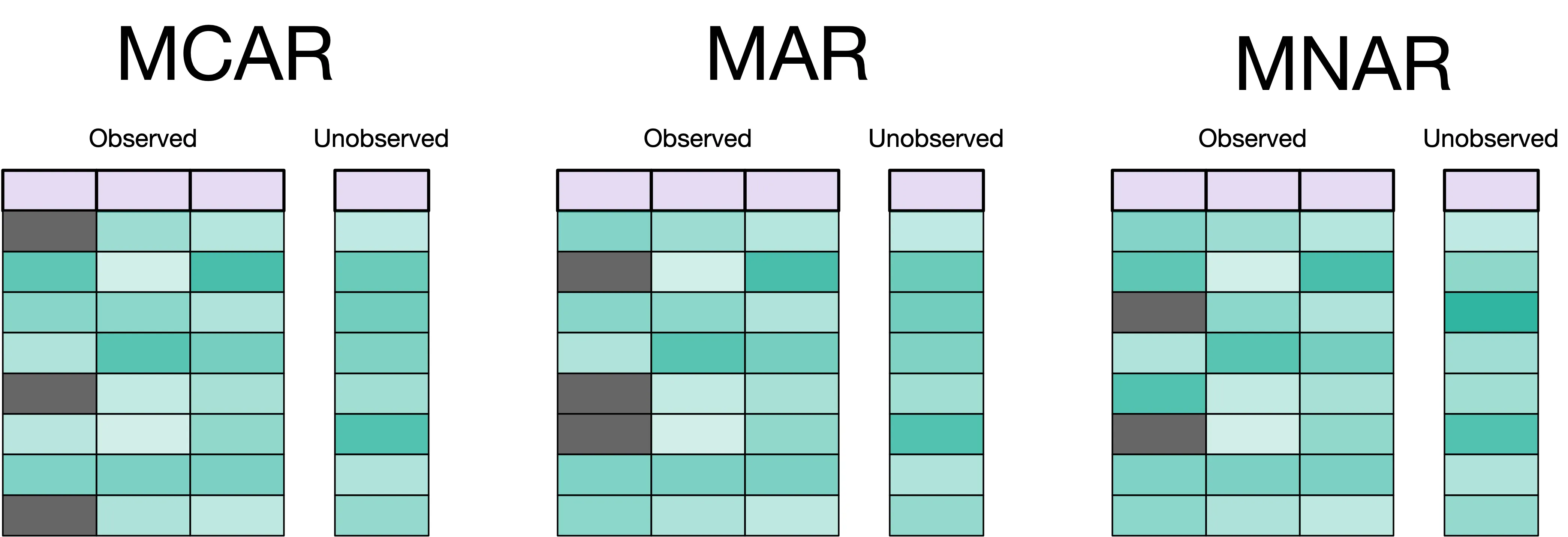
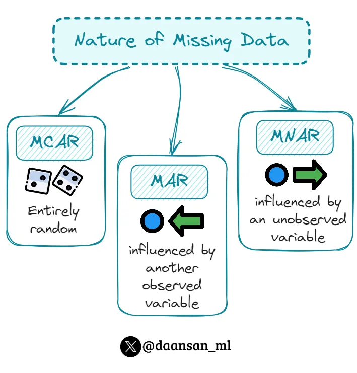Common missing data patterns: MCAR (Missing Completely At Random), MAR (Missing At Random), MNAR (Missing Not At Random)

Data Cleaning Workflow

Missing Data Detection

Missing data detection identifies where data is missing and helps understand the pattern of missingness. This is the first step in any data cleaning process.

Pro tip: Missing data is like that one friend who’s always late to everything - you know they’re supposed to be there, but you can never quite predict when (or if) they’ll show up.

Reference:

df.isnull() - Boolean DataFrame: True for missing values
df.notnull() - Boolean DataFrame: True for non-missing values
df.isna() - Alias for isnull()
df.notna() - Alias for notnull()
df.isnull().sum() - Count missing values per column
df.isnull().any() - True if any missing values in column
df.isnull().all() - True if all values missing in column

Example:

# Check for missing values
df = pd.DataFrame({'A': [1, 2, None, 4], 'B': [5, None, 7, 8]})
print(df.isnull().sum())  # A: 1, B: 1
print(df.isnull().any())  # A: True, B: True
print(df.isnull().all())  # A: False, B: False

# Visualize missing data
import matplotlib.pyplot as plt
df.isnull().sum().plot(kind='bar')
plt.title('Missing Values by Column')
plt.show()

Missing Data Analysis

Missing data analysis helps understand the pattern and mechanism of missingness. This information guides the choice of appropriate handling strategies.

Reference:

df.isnull().sum() - Count missing values per column
df.isnull().sum(axis=1) - Count missing values per row
df.isnull().mean() - Proportion of missing values per column
df.dropna() - Remove rows with any missing values
df.dropna(axis=1) - Remove columns with any missing values
df.dropna(thresh=n) - Keep rows with at least n non-null values

Example:

# Analyze missing data patterns
df = pd.DataFrame({'A': [1, 2, None, 4], 'B': [5, None, 7, 8], 'C': [9, 10, 11, None]})
print(df.isnull().sum())  # Missing values per column
print(df.isnull().mean())  # Proportion missing per column
print(df.isnull().sum(axis=1))  # Missing values per row

# Remove rows with missing values
df_clean = df.dropna()
print(df_clean.shape)  # (2, 3) - removed rows with missing values

Missing Data Imputation

Missing data imputation fills in missing values using various strategies. The choice of imputation method depends on the data type and the pattern of missingness.

Reference:

df.fillna(value) - Fill missing values with constant
df.ffill() / df.fillna(method='ffill') - Forward fill (use previous value; method= deprecated in pandas 3.0)
df.bfill() / df.fillna(method='bfill') - Backward fill (use next value; method= deprecated in pandas 3.0)
df.fillna(df.mean()) - Fill with column mean
df.fillna(df.median()) - Fill with column median
df.fillna(df.mode().iloc[0]) - Fill with column mode
df.interpolate() - Interpolate missing values

Example:

# Fill missing values
df = pd.DataFrame({'A': [1, 2, None, 4], 'B': [5, None, 7, 8]})

# Fill with constant
df_filled = df.fillna(0)
print(df_filled)  # Missing values replaced with 0

# Fill with mean
df_mean = df.fillna(df.mean())
print(df_mean)  # Missing values replaced with column mean

# Forward fill - modern syntax (pandas 1.4+)
df_ffill = df.ffill()
print(df_ffill)  # Missing values replaced with previous value

# Deprecated syntax (still works in pandas 2.x, removed in 3.0)
df_ffill_old = df.fillna(method='ffill')  # Avoid this in new code

Original Data:        Forward Fill (ffill):           Backward Fill (bfill):
  Index Value           Index Value                     Index Value
    0     10              0     10 ─┐                     0     10
    1   [NaN]             1     10 ←┤ fills down          1     15 ←┐
    2   [NaN]             2     10 ←┘ from 10             2     15 ←┤ fills up
    3     15              3     15 ─┐                     3     15 ─┘ from 15
    4   [NaN]             4     15 ←┤ fills down          4   [NaN] can't fill
    5   [NaN]             5     15 ←┘ from 15             5   [NaN] no later rows

LIVE DEMO! (Demo 1: Missing Data - detection, analysis, and imputation strategies)

Data Transformation Techniques

Removing Duplicates

Duplicate rows can skew your analysis and waste computational resources. Removing duplicates is a common first step in data cleaning.

Fun fact: Duplicates are like that one song that gets stuck in your head - they keep showing up everywhere, even when you think you’ve gotten rid of them all.

Reference:

df.duplicated() - Check for duplicate rows
df.drop_duplicates() - Remove duplicate rows
df.drop_duplicates(subset=['col1', 'col2']) - Remove duplicates in specific columns
df.drop_duplicates(keep='first') - Keep first occurrence of duplicates

Example:

# Check for duplicates
df = pd.DataFrame({'A': [1, 2, 2, 3], 'B': [4, 5, 5, 6]})
print(df.duplicated().sum())  # Number of duplicate rows

# Remove duplicates
df_clean = df.drop_duplicates()
print(df_clean)  # Removed duplicate rows

Replacing Values

The replace() method provides a flexible way to substitute specific values or patterns in your data.

Think of replace() as find-and-replace for your data - but way more powerful than Word’s version!

Reference:

df.replace(old, new) - Replace single value
df.replace([val1, val2], new) - Replace multiple values with same replacement
df.replace([val1, val2], [new1, new2]) - Replace multiple values with different replacements
df.replace({val1: new1, val2: new2}) - Dictionary mapping
df.replace(regex=True) - Use regular expressions

Example:

# Replace sentinel values with NaN
df = pd.Series([1, -999, 2, -999, -1000, 3])
df_clean = df.replace([-999, -1000], np.nan)
print(df_clean)  # [1.0, NaN, 2.0, NaN, NaN, 3.0]

# Different replacement for each value
df = pd.Series(['low', 'medium', 'high', 'low'])
df_mapped = df.replace({'low': 1, 'medium': 2, 'high': 3})
print(df_mapped)  # [1, 2, 3, 1]

# Column-specific replacement in DataFrame
df = pd.DataFrame({'A': [1, 2, 3], 'B': ['x', 'y', 'z']})
df = df.replace({'A': {1: 100}, 'B': {'x': 'alpha'}})
print(df)  # A: [100, 2, 3], B: ['alpha', 'y', 'z']

Applying Custom Functions

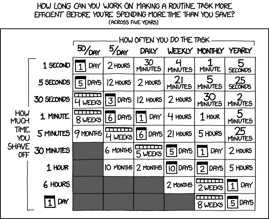xkcd 1205 "Is It Worth the Time?" Classic time-saving calculation chart - perfect for .apply() section

Sometimes built-in methods aren’t enough - you need to apply custom logic to transform your data. The .apply() and .map() methods let you use any function (built-in or custom) to transform data.

Think of .apply() as your data transformation Swiss Army knife - when pandas doesn’t have a built-in method for what you need, you can just write your own function and apply it to every row, column, or value.

Quick lambda primer: A lambda is a one-line anonymous function, perfect for simple transformations: lambda x: x * 2 is equivalent to def double(x): return x * 2, just more concise for one-time use.

Reference:

series.map(dict_or_func) - Map values in a Series (element-wise)
series.apply(func) - Apply function to each element in a Series
df.apply(func, axis=0) - Apply function to each column (axis=0, default)
df.apply(func, axis=1) - Apply function to each row (axis=1)
df.map(func) - Apply function element-wise to entire DataFrame (pandas 2.1+)
df.applymap(func) - Deprecated in pandas 2.1+, use .map() instead

Example:

# Clean text data with custom function
def clean_text(text):
    """Remove whitespace and convert to lowercase"""
    return text.strip().lower()

names = pd.Series(['  Alice  ', 'BOB', '  Charlie'])
names_clean = names.apply(clean_text)
print(names_clean)  # ['alice', 'bob', 'charlie']

# Map categorical values to numbers
status = pd.Series(['active', 'inactive', 'active', 'pending'])
status_map = {'active': 1, 'inactive': 0, 'pending': 2}
status_coded = status.map(status_map)
print(status_coded)  # [1, 0, 1, 2]

# Apply function to DataFrame rows
df = pd.DataFrame({'min': [1, 4, 7], 'max': [5, 9, 12]})
df['range'] = df.apply(lambda row: row['max'] - row['min'], axis=1)
print(df)
#    min  max  range
# 0    1    5      4
# 1    4    9      5
# 2    7   12      5

# Apply function to DataFrame columns
df = pd.DataFrame({'A': [1, 2, 3], 'B': [4, 5, 6]})
column_sums = df.apply(sum, axis=0)  # Sum each column
print(column_sums)  # A: 6, B: 15

# Element-wise function application (pandas 2.1+)
df = pd.DataFrame({'A': [1, 2, 3], 'B': [4, 5, 6]})
df_squared = df.map(lambda x: x ** 2)
print(df_squared)
#    A   B
# 0  1  16
# 1  4  25
# 2  9  36

Data Type Conversion

Converting data to the correct types is essential for proper analysis. This includes converting strings to numbers, dates, and other appropriate types.

Warning: Data type conversion is like trying to fit a square peg in a round hole - sometimes it works perfectly, sometimes you need to shave off a few corners, and sometimes you just need to find a different hole entirely.

Reference:

df.astype('int64') - Convert to integer
df.astype('float64') - Convert to float
df.astype('string') - Convert to string
pd.to_datetime(df['date_column']) - Convert to datetime
pd.to_numeric(df['column'], errors='coerce') - Convert to numeric, errors become NaN

Example:

# Convert data types
df = pd.DataFrame({'A': ['1', '2', '3'], 'B': [4.5, 5.5, 6.5]})
df['A'] = df['A'].astype('int64')  # Convert string to integer
df['B'] = df['B'].astype('int64')  # Convert float to integer
print(df.dtypes)  # A: int64, B: int64

Renaming Axis Indexes

Renaming changes row or column labels without modifying data. This is essential for making your data more readable and standardizing column names.

Reference:

df.rename(index={old: new}) - Rename rows
df.rename(columns={old: new}) - Rename columns
df.rename(columns=str.lower) - Apply function to all columns
df.rename(columns=str.strip) - Remove whitespace from column names
inplace=True - Modify DataFrame in place

Example:

# Rename specific columns
df = pd.DataFrame({'OldName': [1, 2, 3], 'Another_Old': [4, 5, 6]})
df_renamed = df.rename(columns={'OldName': 'new_name', 'Another_Old': 'better_name'})
print(df_renamed.columns)  # ['new_name', 'better_name']

# Apply function to all columns
df.columns = ['First Column', ' Second ', 'THIRD']
df_clean = df.rename(columns=str.lower)  # Lowercase all
df_clean = df_clean.rename(columns=str.strip)  # Remove spaces
print(df_clean.columns)  # ['first column', 'second', 'third']

# Rename index
df.index = ['a', 'b', 'c']
df_reindexed = df.rename(index={'a': 'row_1', 'b': 'row_2'})

Creating Categories

Converting continuous variables into categories makes data easier to analyze and visualize. This is especially useful for age groups, income brackets, and other meaningful categories.

Pro tip: Categories are like putting your data in organized boxes - everything has its place, and you can find things much faster when you know exactly which box to look in.

Reference:

pd.cut(series, bins) - Cut into equal-width bins
pd.qcut(series, q) - Cut into equal-frequency bins
bins=[0, 18, 35, 50, 100] - Custom bin edges
labels=['Young', 'Middle', 'Senior'] - Custom labels for bins

Example:

# Create age groups
ages = pd.Series([25, 30, 45, 60, 75])
age_groups = pd.cut(ages, bins=[0, 30, 50, 100], labels=['Young', 'Middle', 'Senior'])
print(age_groups)  # [Young, Young, Middle, Senior, Senior]

Detecting and Filtering Outliers

Outliers are extreme values that may represent errors or important anomalies. Detecting and handling them appropriately is crucial for reliable analysis.

IQR Method for Outlier Detection

Reference:

df[df['col'] > threshold] - Filter by threshold
df.clip(lower, upper) - Cap values at bounds
df.quantile([0.25, 0.75]) - Find quartiles for IQR method
df[(df > lower) & (df < upper)] - Filter within bounds

Example:

# Remove values beyond 3 standard deviations
df = pd.DataFrame({'value': [1, 2, 3, 100, 4, 5]})
mean, std = df['value'].mean(), df['value'].std()
df_clean = df[abs(df['value'] - mean) < 3 * std]
print(df_clean)  # Removes 100

# Cap extreme values
df['value'] = df['value'].clip(lower=0, upper=10)
print(df)  # Values capped at 0-10 range

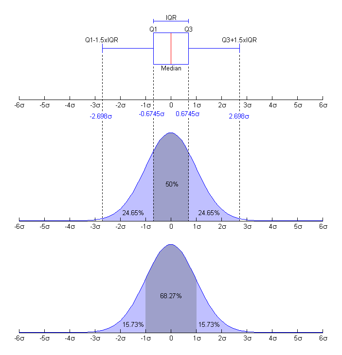
# IQR method for outlier detection
Q1 = df['value'].quantile(0.25)
Q3 = df['value'].quantile(0.75)
IQR = Q3 - Q1
lower_bound = Q1 - 1.5 * IQR
upper_bound = Q3 + 1.5 * IQR
df_no_outliers = df[(df['value'] >= lower_bound) & (df['value'] <= upper_bound)]

Categorical Data Encoding

Working with categorical data is common in data analysis. Pandas provides two main approaches: the categorical data type for efficient storage, and dummy variables for machine learning models.

Pro tip: Categorical encoding is like translating between languages - categories can be stored efficiently as codes (integers) or expanded into binary columns for models. Choose the right translation for your task!

Categorical Data Type

The categorical type is incredibly powerful for memory optimization, especially when you have repeated string values.

Visual showing categorical encoding: Original values → Categories → Codes with memory savings comparison

Reference:

astype('category') - Convert to categorical
cat.categories - View categories
cat.codes - View numeric codes
Use for: Repeated string values, ordered categories

Example:

# Huge memory savings for repeated values
colors = pd.Series(['red', 'blue', 'red', 'green', 'blue'] * 1000)
print(f"As object: {colors.memory_usage(deep=True)} bytes")

colors_cat = colors.astype('category')
print(f"As category: {colors_cat.memory_usage(deep=True)} bytes")

# Access categories and codes
print(colors_cat.cat.categories)  # ['blue', 'green', 'red']
print(colors_cat.cat.codes[:5])   # [2, 0, 2, 1, 0]

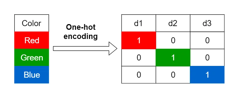
Creating Indicator (Dummy) Variables

Indicator variables convert categories into binary (0/1) columns, which is essential for machine learning models that require numeric input.

Think of dummy variables as translating categories into a language that models can understand - instead of “red”, “blue”, “green”, you get three columns of 1s and 0s indicating which color each row has.

Reference:

pd.get_dummies(series) - Create dummy variables
prefix='category' - Add prefix to column names
drop_first=True - Avoid multicollinearity (drop first category)
dtype='int64' - Specify data type for dummies (use int64 not bool - booleans can’t represent missing values)

Example:

# Create dummy variables
df = pd.DataFrame({'color': ['red', 'blue', 'red', 'green']})
dummies = pd.get_dummies(df['color'], prefix='color', dtype='int64')
print(dummies)
# Creates: color_blue, color_green, color_red columns with 0/1 values

# Add to original DataFrame
df_with_dummies = pd.concat([df, dummies], axis=1)
print(df_with_dummies)

# Drop first category to avoid multicollinearity
dummies = pd.get_dummies(df['color'], prefix='color', drop_first=True, dtype='int64')
print(dummies)  # Only color_green and color_red (blue is the reference)

LIVE DEMO! (Demo 2: Transformations - categorical encoding, string operations, sampling)

String Manipulation

Pro tip: The .str accessor is like having a Swiss Army knife for text data. It can split, join, replace, extract, and transform text in ways that would make a regex wizard jealous.

Basic String Operations

String operations are essential for cleaning text data. Pandas provides easy-to-use string methods that work on Series containing text.

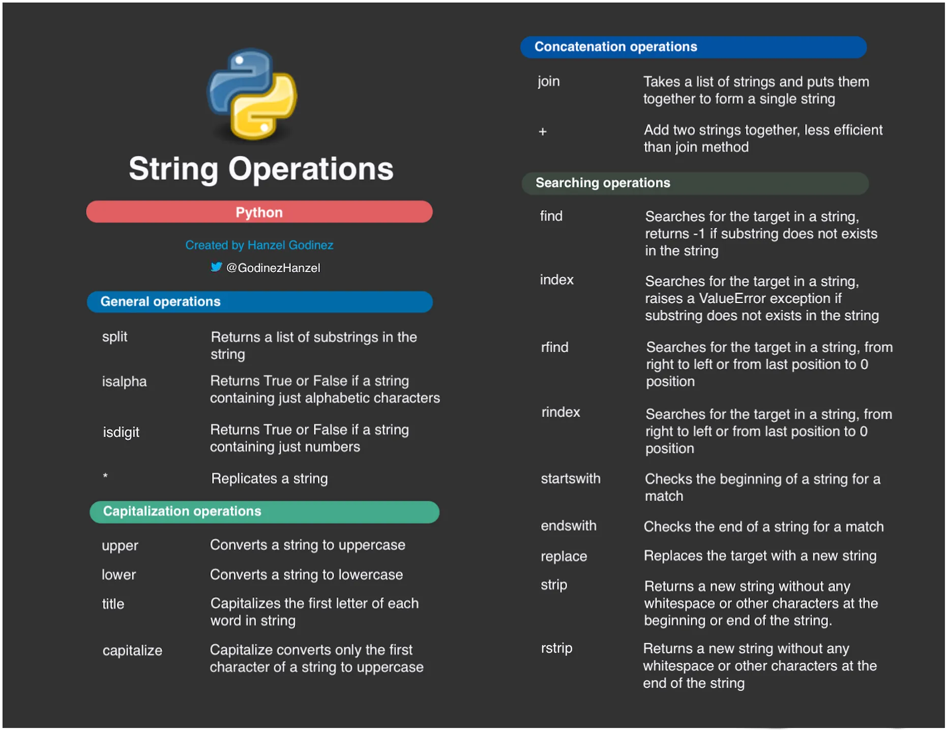String Operations Reference Quick reference card for common string operations: .upper()/.lower(), .strip()/.replace(), .split()/.contains()

Input: "  Alice Smith  "
   │
   ├─ .strip() ────────────► "Alice Smith"
   │                              │
   │                              ├─ .lower() ────────► "alice smith"
   │                              │                          │
   │                              │                          └─ .replace(' ', '_') ──► "alice_smith"
   │                              │
   │                              └─ .split(' ') ────────► ['Alice', 'Smith']
   │                                     │
   │                                     └─ [0] ──────────► 'Alice'
   │
   └─ .title() ────────────► "Alice Smith"

xkcd 1171 "Perl Problems" “I got 99 problems, so I used regex. Now I have 100 problems.” - Perfect humor for string manipulation complexity

Reference:

series.str.upper() - Convert to uppercase
series.str.lower() - Convert to lowercase
series.str.strip() - Remove leading/trailing whitespace
series.str.replace(old, new) - Replace substrings
series.str.contains(pattern) - Check if string contains pattern
series.str.startswith(prefix) - Check if string starts with prefix
series.str.endswith(suffix) - Check if string ends with suffix

Example:

# Clean text data
names = pd.Series(['  Alice  ', 'bob', 'CHARLIE'])
clean_names = names.str.strip().str.title()
print(clean_names)  # ['Alice', 'Bob', 'Charlie']

# Check patterns
emails = pd.Series(['alice@example.com', 'bob@test.org'])
has_gmail = emails.str.contains('gmail')
print(has_gmail)  # [False, False]

String Splitting and Joining

Splitting and joining strings is common when working with structured text data like addresses, names, or delimited values.

Reference:

series.str.split(sep) - Split strings by separator
series.str.split(sep, expand=True) - Split into separate columns
series.str.cat(sep=' ') - Join strings with separator
series.str.join(sep) - Join list elements with separator

Example:

# Split strings
full_names = pd.Series(['Alice Smith', 'Bob Jones', 'Charlie Brown'])
names_split = full_names.str.split(' ')
print(names_split)  # [['Alice', 'Smith'], ['Bob', 'Jones'], ['Charlie', 'Brown']]

# Split into columns
names_df = full_names.str.split(' ', expand=True)
print(names_df)  # Two columns with first and last names

Random Sampling and Permutation

Random Sampling

Random sampling creates representative subsets of data for analysis, testing, and machine learning. It’s essential for creating train/test splits, bootstrap analysis, and data exploration.

Reference:

df.sample(n=None, frac=None, replace=False, weights=None, random_state=None) - Random sampling
n=10 - Sample exactly 10 rows
frac=0.5 - Sample 50% of rows
replace=True - Sample with replacement (bootstrap)
weights='column' - Weighted sampling by column values
random_state=42 - Reproducible sampling
df.iloc[::step] - Systematic sampling every nth row

Example:

# Random sampling
df = pd.DataFrame({'A': range(100), 'B': range(100, 200)})
sample = df.sample(n=10, random_state=42)  # Sample 10 rows
print(len(sample))  # 10

# Stratified sampling
df['category'] = ['A', 'B'] * 50
stratified = df.groupby('category').apply(lambda x: x.sample(2))
print(len(stratified))  # 4 (2 from each category)

Permutation and Shuffling

Permutation randomizes data order while preserving relationships. It’s essential for cross-validation, bootstrap analysis, and breaking temporal dependencies in time series data.

Reference:

df.sample(frac=1) - Shuffle all rows (permutation)
df.reindex(np.random.permutation(df.index)) - Permute index order
df.sample(n=len(df), replace=True) - Bootstrap sampling
np.random.permutation(array) - Randomly permute array
random_state=42 - Reproducible permutation

Example:

# Shuffle DataFrame
df = pd.DataFrame({'A': [1, 2, 3, 4], 'B': [5, 6, 7, 8]})
shuffled = df.sample(frac=1, random_state=42)
print(shuffled)  # Random order of rows

# Bootstrap sampling
bootstrap = df.sample(n=len(df), replace=True, random_state=42)
print(len(bootstrap))  # 4 (same length, but with replacement)

Data Validation and Quality Assessment

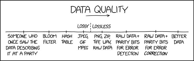xkcd 2239 "Database" Shows data errors invalidating research - perfect for validation section

Issue	Detection	Solution
Missing Values	`df.isnull().sum()`	• Impute (mean/median) • Forward/backward fill • Drop if <5% missing
Duplicates	`df.duplicated()`	• `drop_duplicates()` • Keep first or last
Wrong Data Type	`df.dtypes`	• `astype('int64')` • `pd.to_datetime()`
Outliers	`df.describe()` Box plots	• IQR method filter • Clip extreme values • Keep if valid (verify)
Inconsistent Categories	`df['col'].unique()`	• `str.lower().strip()` • `replace()` mapping

Data Quality Checks

Data quality checks identify issues like missing values, duplicates, outliers, and data type inconsistencies. These checks are essential for ensuring reliable analysis results.

Reference:

df.isnull().sum() - Count missing values per column
df.duplicated().sum() - Count duplicate rows
df.nunique() - Count unique values per column
df.dtypes - Data types per column
df.describe() - Summary statistics (numeric columns only by default)
df.describe(include='all') - Summary statistics for all columns (numeric + categorical)
df.describe(include=['object']) - Summary statistics for categorical columns only
df.info() - Detailed information
df.memory_usage() - Memory usage per column

Example:

# Data quality assessment
df = pd.DataFrame({'A': [1, 2, 2, 4], 'B': [5, 6, 6, 8], 'C': [9, 10, 11, 12]})
print(df.isnull().sum())  # Missing values per column
print(df.duplicated().sum())  # Number of duplicate rows
print(df.nunique())  # Unique values per column
print(df.dtypes)  # Data types per column

Data Validation Rules

Data validation rules ensure data meets business requirements and constraints. These rules help maintain data integrity and prevent analysis errors.

Reference:

df[condition] - Filter rows meeting condition
df.between(left, right) - Check if values are between bounds
df.isin(values) - Check if values are in list
df.str.contains(pattern) - Check if strings contain pattern
df.str.match(pattern) - Check if strings match pattern
df.str.len() - Get string length
df.str.isdigit() - Check if strings are digits

Example:

# Data validation rules
df = pd.DataFrame({'Age': [25, 30, 35, 40], 'Email': ['alice@test.com', 'bob@example.org', 'charlie@test.com', 'diana@example.org']})

# Age validation (18-65)
valid_ages = df[df['Age'].between(18, 65)]
print(valid_ages)  # All rows (ages are valid)

# Email validation
email_pattern = r'^[a-zA-Z0-9._%+-]+@[a-zA-Z0-9.-]+\.[a-zA-Z]{2,}$'
valid_emails = df[df['Email'].str.match(email_pattern)]
print(valid_emails)  # All rows (emails are valid)

Data Cleaning Pipeline

A systematic approach to data cleaning ensures consistent, high-quality results. Follow these steps in order for best results.

graph TD
    A[Load Data] --> B{Inspect Data}
    B --> C[Check Missing Values]
    B --> D[Check Duplicates]
    B --> E[Check Data Types]
    B --> F[Check Outliers]

    C --> G{Issues Found?}
    D --> G
    E --> G
    F --> G

    G -->|Yes| H[Handle Issues]
    G -->|No| L[Validate Results]

    H --> I[Fill/Drop Missing]
    H --> J[Remove Duplicates]
    H --> K[Convert Types]
    H --> M[Handle Outliers]

    I --> L
    J --> L
    K --> L
    M --> L

    L --> N{Data Quality OK?}
    N -->|No| B
    N -->|Yes| O[Document Decisions]
    O --> P[Export Clean Data]

Think of data cleaning as being a detective - you need to follow the clues, ask the right questions, and sometimes you have to make tough decisions about what to keep and what to throw away.

Reference:

Load and inspect data - df.head(), df.info(), df.describe()
Handle missing values - df.isnull().sum(), df.fillna(), df.dropna()
Remove duplicates - df.duplicated(), df.drop_duplicates()
Convert data types - df.astype(), pd.to_datetime(), pd.to_numeric()
Handle outliers - df.quantile(), df.clip(), filtering
Validate data quality - Check ranges, patterns, consistency
Export clean data - df.to_csv(), df.to_excel()

Example:

# Step 1: Load and inspect
df = pd.read_csv('messy_data.csv')
print(df.info())
print(df.isnull().sum())

# Step 2: Handle missing values
df['Age'].fillna(df['Age'].mean(), inplace=True)
df['Name'].fillna('Unknown', inplace=True)

# Step 3: Remove duplicates
df = df.drop_duplicates()

# Step 4: Convert data types
df['Age'] = df['Age'].astype('int64')
df['Date'] = pd.to_datetime(df['Date'])

# Step 5: Handle outliers
Q1, Q3 = df['Salary'].quantile([0.25, 0.75])
IQR = Q3 - Q1
df = df[~((df['Salary'] < Q1 - 1.5*IQR) | (df['Salary'] > Q3 + 1.5*IQR))]

# Step 6: Validate
print(df.describe())
print(df.dtypes)

# Step 7: Export
df.to_csv('clean_data.csv', index=False)

Configuration-Driven Processing

Configuration files make data cleaning pipelines more maintainable and reproducible. Simple text files or Python dictionaries can store filter rules, cleaning parameters, and processing steps.

Pro tip: Keep your data cleaning logic separate from your parameters. This makes your code more maintainable and your pipelines more reproducible.

Reference:

Use Python dictionaries for simple configurations
Store parameters in separate files (CSV, JSON, or simple text)
Keep cleaning logic in functions
Document your cleaning decisions

Example:

# Simple configuration dictionary
cleaning_config = {
    'missing_strategies': {
        'age': 'median',
        'income': 'mean',
        'date': 'ffill'
    },
    'outlier_threshold': 3.0,
    'drop_columns': ['temp_id', 'notes']
}

# Apply configuration
for column, strategy in cleaning_config['missing_strategies'].items():
    if strategy == 'median':
        df[column].fillna(df[column].median(), inplace=True)
    elif strategy == 'mean':
        df[column].fillna(df[column].mean(), inplace=True)
    elif strategy == 'ffill':
        df[column].fillna(method='ffill', inplace=True)

Running Notebooks from Command Line

For automated pipelines and batch processing, you can execute Jupyter notebooks from the command line without opening the Jupyter interface.

Basic Execution

# Execute a single notebook
jupyter nbconvert --execute --to notebook your_notebook.ipynb

# Execute and save output to a new file
jupyter nbconvert --execute --to notebook --output executed_notebook your_notebook.ipynb

# Execute and overwrite the original file
jupyter nbconvert --execute --to notebook --inplace your_notebook.ipynb

Notebook Pipeline Automation

Always check “exit codes” after notebook execution to ensure your pipeline stops if any step fails. When a command runs successfully it returns an exit code of 0, other values (usually 1) indicate an error.

You may check exit codes using the special variable $?, which contains exit code for the previous command. Alternatively, we can use an OR operator (||) to instruct the shell to do something when a command fails.

Note: The || operator means “OR” - if the command fails (non-zero exit code), execute the code block in curly braces {}. This is more concise than checking $? explicitly.

#!/bin/bash
# Example pipeline script

echo "Starting data analysis pipeline..."

# Run notebooks in sequence
jupyter nbconvert --execute --to notebook q4_exploration.ipynb
if [ $? -ne 0 ]; then
    echo "ERROR: Q4 exploration failed"
    exit 1
fi

jupyter nbconvert --execute --to notebook q5_missing_data.ipynb || {
    echo "ERROR: Q5 missing data analysis failed"
    exit 1
}

echo "Pipeline completed successfully!"

Key Parameters

--execute: Run all cells in the notebook
--to notebook: Keep output as notebook format
--inplace: Overwrite the original file
--output filename: Save to a new file
--allow-errors: Continue execution even if cells fail

LIVE DEMO!

(Demo 3: Complete Workflow - end-to-end data cleaning pipeline)