07: Data Cleaning

See Bonus for advanced topics:

• Advanced matplotlib customization and publication-quality plots
• Interactive visualization with Bokeh and Plotly
• Statistical visualization with seaborn advanced features
• Custom color palettes and themes
• Animation and dynamic plots

Fun fact: The word “visualization” comes from the Latin “visus” meaning “sight.” In data science, we’re literally making data visible - turning numbers into stories that our eyes can understand and our brains can process.

Outline

• matplotlib fundamentals (figures, subplots, customization)
• Statistical visualizations with seaborn
• pandas plotting for quick data exploration
• Visualization principles and best practices
• Tufte’s principles for effective data visualization
• Modern visualization libraries (altair, plotnine)

“The data clearly shows that our hypothesis is correct, assuming we ignore all the data that doesn’t support our hypothesis.”

Edward Tufte’s Principles of Data Visualization

Good visualization is like good writing - it should be clear, honest, and serve the reader (or viewer) first.

“Above all else, show the data.” - Edward Tufte

Edward Tufte, the pioneer of information design, established fundamental principles that remain essential for effective data visualization.

Essential Reading:

• The Visual Display of Quantitative Information - Tufte’s seminal work
• Envisioning Information - Color, layering, and detail
• Tufte’s website - Essays and resources

1. Data-Ink Ratio: Maximize the Data-Ink

The data-ink ratio is the proportion of ink (or pixels) used to present actual data compared to the total ink used in the entire display.

Data-Ink Ratio = Data-Ink / Total Ink Used

Tufte’s Goal: Maximize this ratio by eliminating non-data ink (chartjunk).

Key Practices:

• Remove unnecessary gridlines (or make them subtle)
• Eliminate decorative elements that don’t convey information
• Use direct labeling instead of legends when possible
• Avoid 3D effects and shadows that distort perception
• Remove redundant labels and tick marks

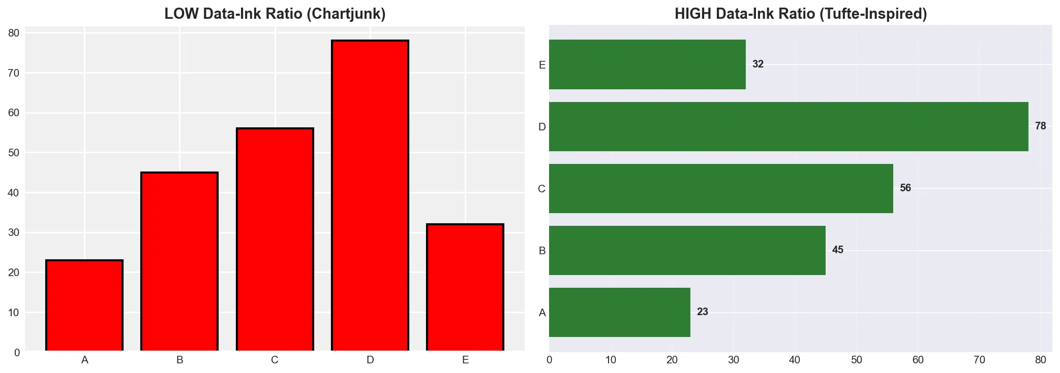
Left: Low data-ink ratio with excessive decoration. Right: High data-ink ratio focusing on the data.

2. Chartjunk: Eliminate Visual Noise

Chartjunk includes any visual elements that do not convey information:

• Unnecessary 3D effects
• Heavy grid lines
• Decorative fills and patterns
• Excessive colors
• Redundant labels

3. Lie Factor: Maintain Visual Integrity

The lie factor measures how much a visualization distorts the data:

Lie Factor = (Size of effect shown in graphic) / (Size of effect in data)

Ideal Lie Factor: Close to 1.0 (no distortion)

Common distortions to avoid:

• Truncated y-axes that exaggerate differences
• 3D perspective that distorts area/volume comparisons
• Inconsistent scales
• Cherry-picked time ranges

4. Small Multiples: Show Comparisons

Use small, repeated charts with the same scale to enable easy comparison across categories or time.

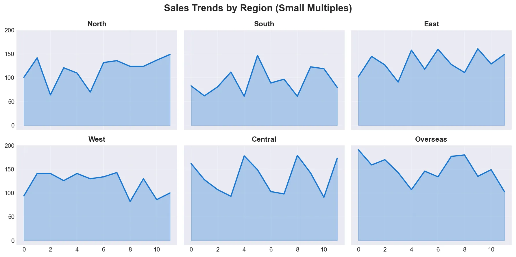
Small multiples enable quick visual comparison across multiple dimensions while maintaining consistent scales.

5. High-Resolution Data Graphics

Show as much detail as the data allows - don’t oversimplify or aggregate unnecessarily.

Before/After Examples: Applying Tufte’s Principles

Example 1: Bar Chart Redesign

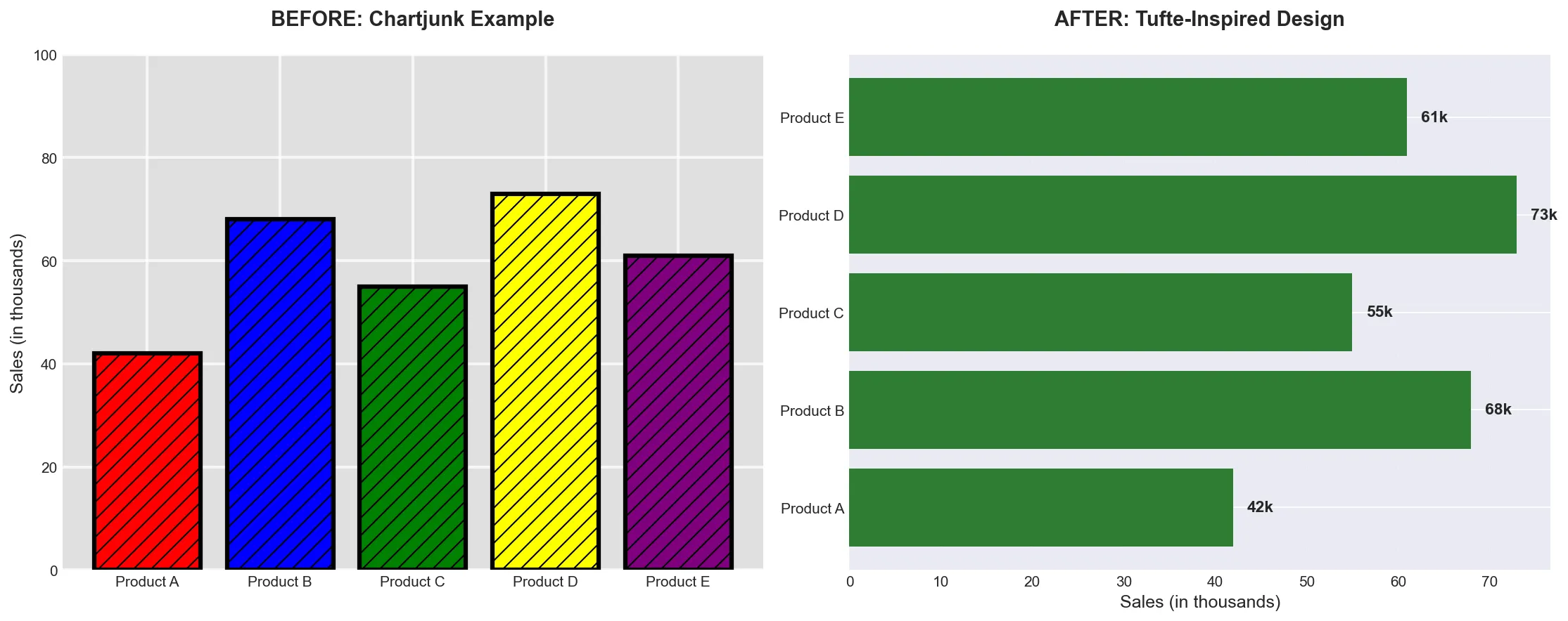
Before (left): Excessive colors, patterns, and heavy gridlines distract from the data. After (right): Clean design with direct labeling maximizes data-ink ratio.

Example 2: Line Chart with Truncated Axis (Lie Factor)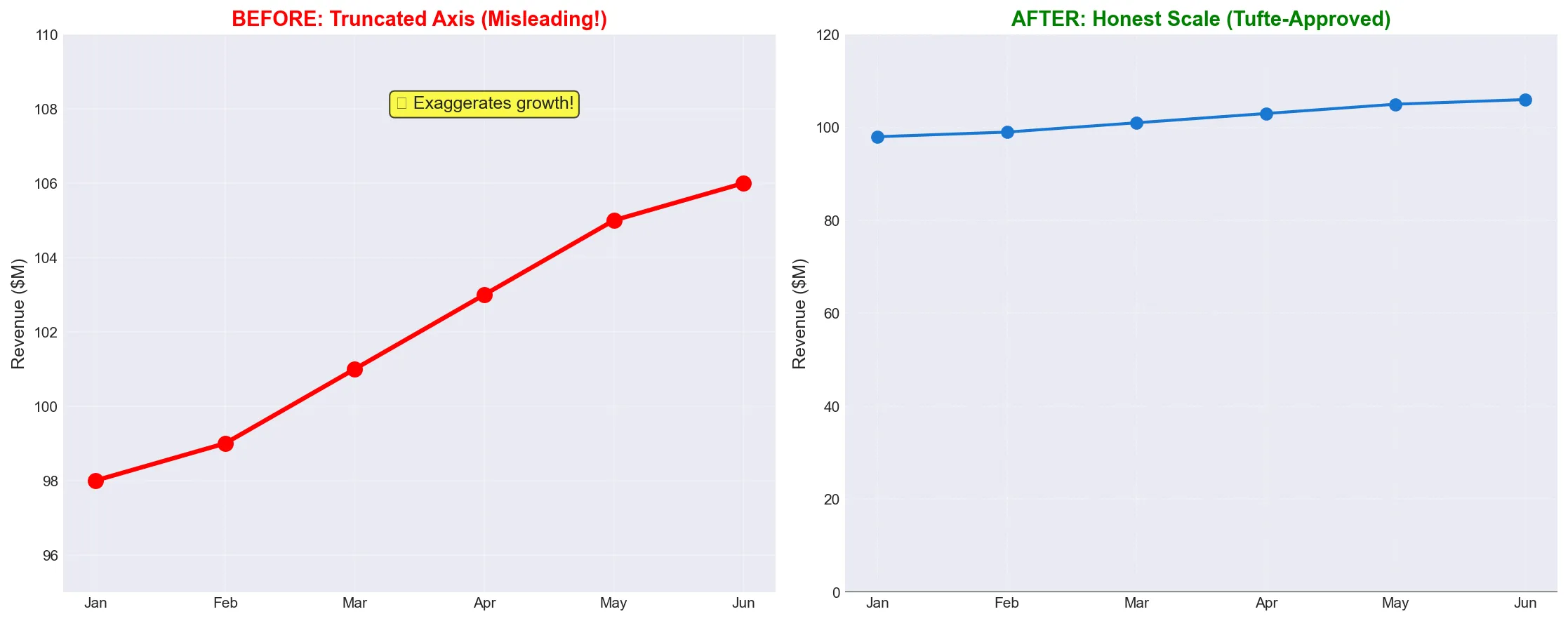

Before (left): Truncated y-axis creates a high lie factor, exaggerating modest growth. After (right): Honest scale starting at zero shows true magnitude of change.

Color Palette Best Practices

Different data types require different color strategies:

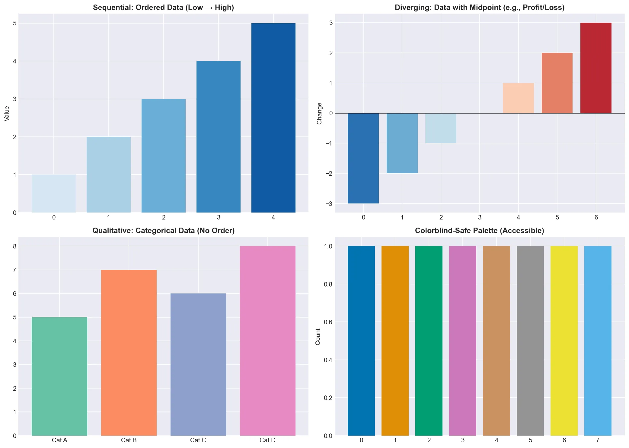
Color Selection Guidelines:

• Sequential: Use for ordered data (temperature, age, income) - single hue gradient
• Diverging: Use for data with meaningful zero/midpoint (profit/loss, correlation) - two contrasting hues
• Qualitative: Use for categories with no inherent order - distinct, unrelated colors
• Accessibility: Always test for colorblind accessibility using tools like ColorBrewer

Additional Resources:

• ColorBrewer 2.0 - Interactive color advice for maps and visualizations
• Colorblind-Safe Palettes - Paul Tol’s color schemes
• Adobe Color - Create and explore color schemes

The Right Chart for the Job

Chart Selection Guide:

• Line charts: Time series, trends over time
• Bar charts: Categories, comparisons
• Scatter plots: Relationships between two variables
• Histograms: Distribution of single variable
• Box plots: Distribution with outliers
• Heatmaps: Patterns in 2D data
• Pie charts: Parts of a whole (use sparingly!)

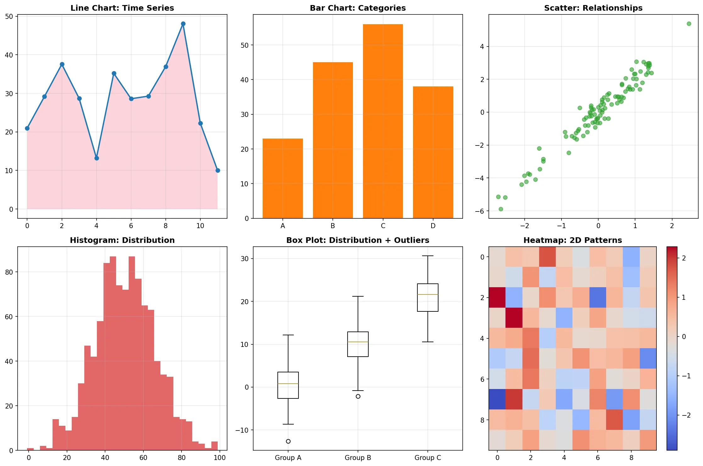
Different chart types are optimized for different data relationships and questions. Choose the right chart for your message.

The Visualization Ecosystem

Reality check: There are more Python visualization libraries than there are ways to mess up a bar chart. But don’t worry - we’ll focus on the essential tools that actually matter for daily data science work.

Python’s visualization landscape has evolved dramatically. While matplotlib remains the foundation, modern tools like seaborn, altair, and plotnine offer more intuitive interfaces for common tasks.

Visual Guide - Python Visualization Stack:

FOUNDATION LAYER
┌─────────────────────────────────────┐
│           matplotlib                │  ← Low-level, highly customizable
│     (The foundation of everything)   │
└─────────────────────────────────────┘
                    ↑
                    │
            PANDAS LAYER
┌─────────────────────────────────────┐
│         pandas.plot()              │  ← Quick exploration, built on matplotlib
│     (DataFrame/Series plotting)     │
└─────────────────────────────────────┘
                    ↑
                    │
            STATISTICAL LAYER
┌─────────────────────────────────────┐
│           seaborn                   │  ← Statistical plots, beautiful defaults
│     (Built on matplotlib)           │
└─────────────────────────────────────┘
                    ↑
                    │
            MODERN LAYER
┌─────────────────────────────────────┐
│    altair (vega-lite)               │  ← Grammar of graphics, interactive
│    plotnine (ggplot2)               │  ← R's ggplot2 in Python
└─────────────────────────────────────┘

Choosing the Right Tool

When to use what:

• pandas.plot() - Quick exploration, basic charts
• matplotlib - Custom plots, publication quality, fine control
• seaborn - Statistical plots, beautiful defaults, relationship analysis
• altair - Interactive plots, grammar of graphics, web-ready
• plotnine - If you know ggplot2, consistent API

Pro tip: Start with pandas for exploration, seaborn for analysis, matplotlib for customization, and modern tools for interactive/sharing needs.

matplotlib: Foundation Layer

Think of matplotlib as the foundation of your visualization house - you can build anything on it, but you need to understand the plumbing before you can install the fancy fixtures.

matplotlib is the bedrock of Python visualization. While it can be verbose, understanding its core concepts gives you the power to create any visualization you can imagine.

Figures and Subplots

Every matplotlib plot lives within a Figure object, which can contain multiple subplots (individual plot areas).

Reference:

• plt.figure(figsize=(width, height)) - Create a new figure
• fig.add_subplot(rows, cols, position) - Add subplot to figure
• plt.subplots(rows, cols) - Create figure with multiple subplots
• fig.savefig('filename.png', dpi=300) - Save figure to file
• plt.show() - Display the plot

Example:

import matplotlib.pyplot as plt
import numpy as np

# Create a figure with 2x2 subplots
fig, axes = plt.subplots(2, 2, figsize=(10, 8))

# Plot on each subplot
axes[0, 0].plot([1, 2, 3, 4], [1, 4, 2, 3])
axes[0, 0].set_title('Line Plot')

axes[0, 1].hist(np.random.normal(0, 1, 1000), bins=30)
axes[0, 1].set_title('Histogram')

axes[1, 0].scatter(np.random.randn(100), np.random.randn(100))
axes[1, 0].set_title('Scatter Plot')

axes[1, 1].bar(['A', 'B', 'C'], [3, 7, 2])
axes[1, 1].set_title('Bar Chart')

plt.tight_layout()
plt.show()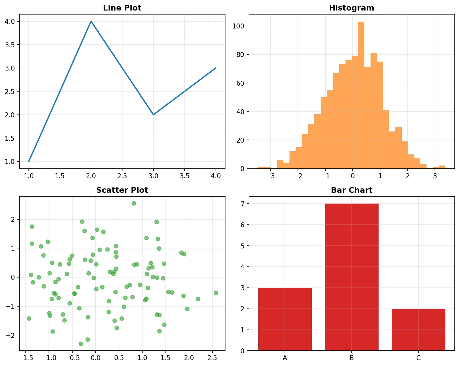

Creating multiple subplots in a single figure allows for easy comparison across different visualization types.

Customizing Plots

matplotlib’s power comes from its extensive customization options.

Reference:

• ax.set_title('Title') - Set plot title
• ax.set_xlabel('X Label') - Set x-axis label
• ax.set_ylabel('Y Label') - Set y-axis label
• ax.set_xlim(min, max) - Set x-axis limits
• ax.set_ylim(min, max) - Set y-axis limits
• ax.grid(True) - Add grid lines
• ax.legend() - Add legend
• ax.set_style('seaborn') - Change plot style

Example:

# Create a customized plot
fig, ax = plt.subplots(figsize=(8, 6))

# Generate sample data
x = np.linspace(0, 10, 100)
y1 = np.sin(x)
y2 = np.cos(x)

# Plot with customization
ax.plot(x, y1, label='sin(x)', color='blue', linewidth=2)
ax.plot(x, y2, label='cos(x)', color='red', linewidth=2, linestyle='--')

# Customize appearance
ax.set_title('Trigonometric Functions')
ax.set_xlabel('X values')
ax.set_ylabel('Y values')
ax.grid(True, alpha=0.3)
ax.legend()

plt.tight_layout()
plt.show()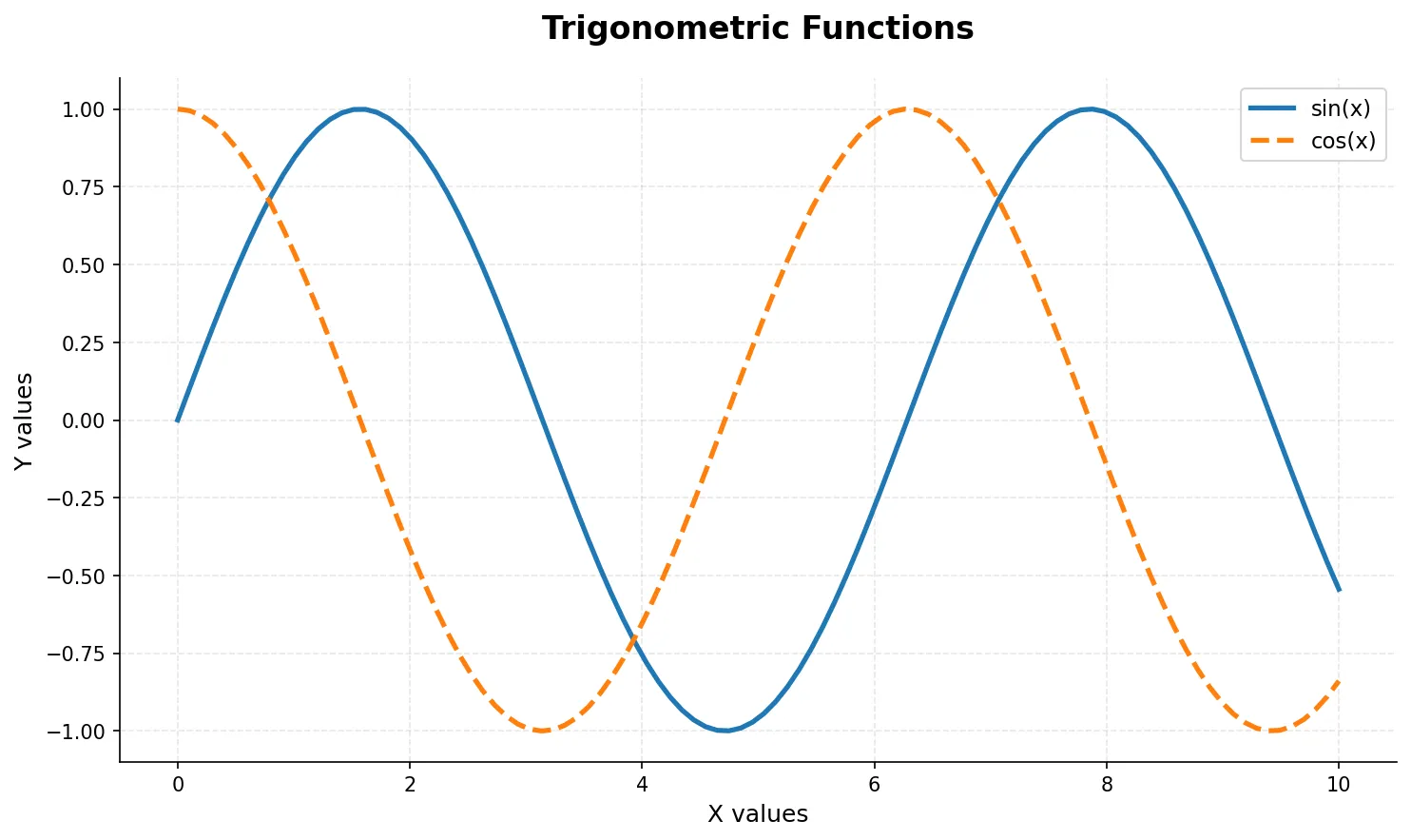

Customization allows you to create publication-quality plots with precise control over every visual element.

Colors, Markers, and Line Styles

matplotlib offers extensive control over visual elements.

Reference:

Colors:

• Named colors: 'red', 'blue', 'green'
• Hex colors: '#FF5733', '#2E8B57'
• RGB tuples: (0.1, 0.2, 0.5)

Line Styles:

• '-' solid, '--' dashed, '-.' dash-dot, ':' dotted

Markers:

• 'o' circle, 's' square, '^' triangle, '*' star

Example:

# Demonstrate different styles
fig, ax = plt.subplots(figsize=(10, 6))

x = np.linspace(0, 10, 20)

# Different line styles and markers
ax.plot(x, x, 'o-', label='circles', color='blue', markersize=8)
ax.plot(x, x**0.5, 's--', label='squares', color='red', markersize=6)
ax.plot(x, np.log(x+1), '^-.', label='triangles', color='green', markersize=8)
ax.plot(x, np.sin(x), '*:', label='stars', color='purple', markersize=10)

ax.set_title('Different Line Styles and Markers')
ax.legend()
ax.grid(True, alpha=0.3)
plt.show()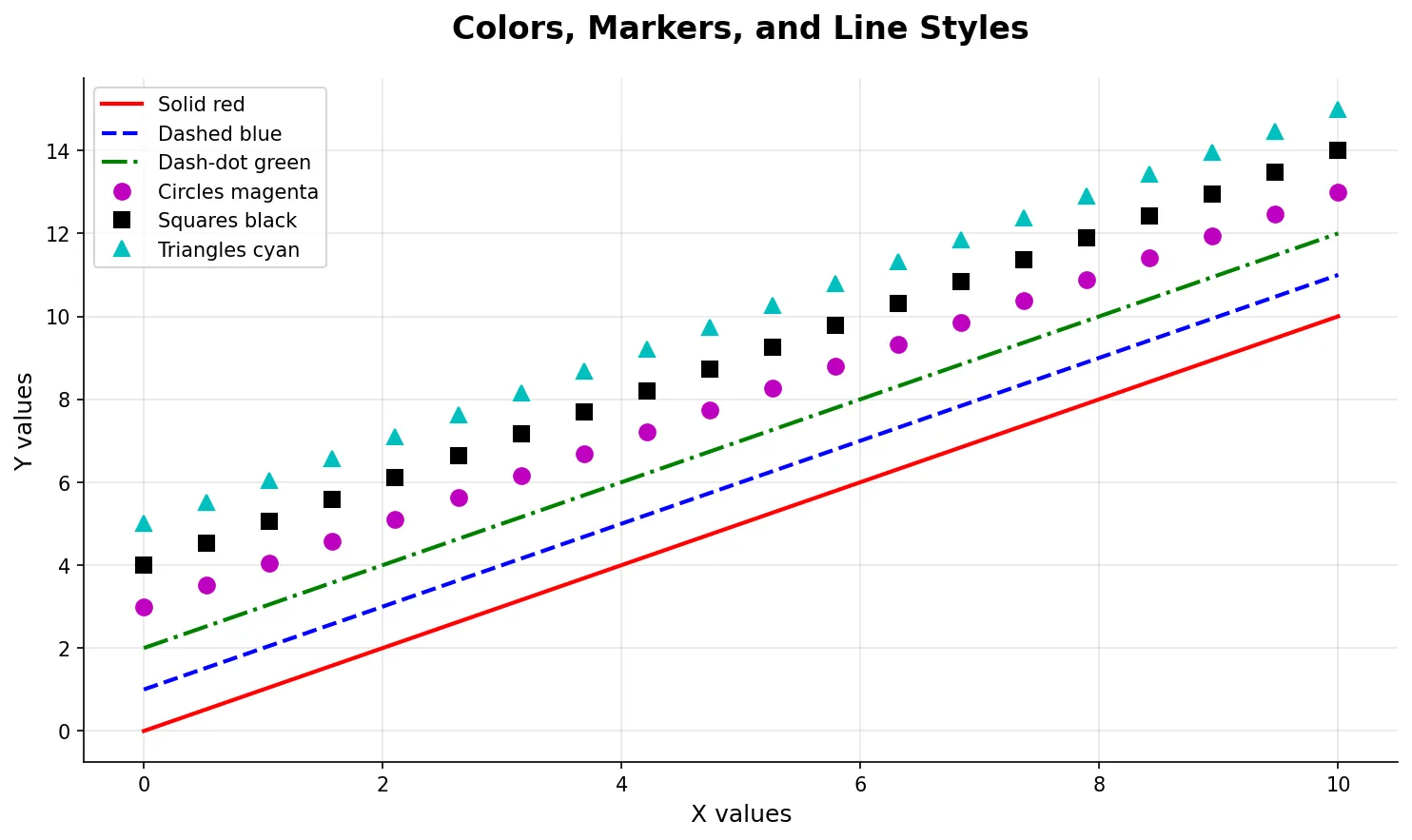

matplotlib provides extensive options for colors, markers, and line styles to create visually distinct data series.

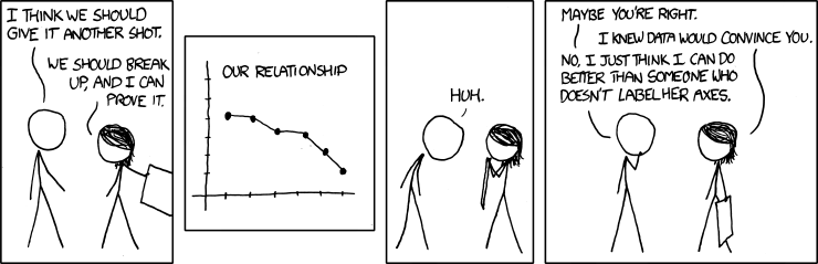
“And if you don’t label your axes, I’m leaving you.” - The importance of proper chart labeling, illustrated.

LIVE DEMO!

pandas: Quick Data Exploration

Think of pandas plotting as your data exploration Swiss Army knife - not the most specialized tool, but incredibly useful for getting a quick sense of your data.

pandas provides convenient plotting methods that build on matplotlib, perfect for quick data exploration.

Reference:

• df.plot() - Line plot (default)
• df.plot(kind='bar') - Bar chart
• df.plot(kind='hist') - Histogram
• df.plot(kind='scatter', x='col1', y='col2') - Scatter plot
• df.plot(kind='box') - Box plot
• df.plot(kind='pie') - Pie chart

Example:

import pandas as pd
import numpy as np

# Create sample data
np.random.seed(42)
df = pd.DataFrame({
    'A': np.random.randn(100),
    'B': np.random.randn(100),
    'C': np.random.randn(100)
})

# Quick exploration with pandas
fig, axes = plt.subplots(2, 2, figsize=(12, 10))

# Line plot
df.plot(ax=axes[0, 0], title='Line Plot')

# Histogram
df.plot(kind='hist', ax=axes[0, 1], alpha=0.7, title='Histogram')

# Scatter plot
df.plot(kind='scatter', x='A', y='B', ax=axes[1, 0], title='Scatter Plot')

# Box plot
df.plot(kind='box', ax=axes[1, 1], title='Box Plot')

plt.tight_layout()
plt.show()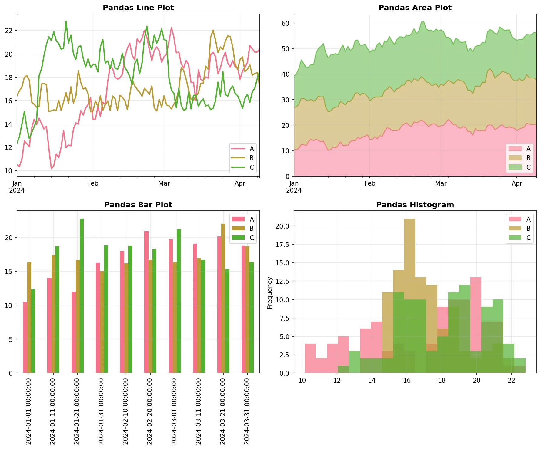

pandas plotting methods provide quick, convenient visualization for data exploration with minimal code.

DataFrame Plotting Options

Reference:

• subplots=True - Create separate subplots for each column
• figsize=(width, height) - Set figure size
• title='Title' - Set plot title
• xlabel='X Label' - Set x-axis label
• ylabel='Y Label' - Set y-axis label
• legend=True - Show legend
• grid=True - Add grid lines

Example:

# Sales data example
sales_data = pd.DataFrame({
    'Month': ['Jan', 'Feb', 'Mar', 'Apr', 'May', 'Jun'],
    'Product_A': [100, 120, 110, 130, 140, 135],
    'Product_B': [80, 90, 95, 105, 110, 115],
    'Product_C': [60, 70, 75, 80, 85, 90]
})

# Set Month as index for better plotting
sales_data.set_index('Month', inplace=True)

# Create subplots for each product
sales_data.plot(subplots=True, figsize=(10, 8),
                title='Sales by Product Over Time',
                grid=True, legend=True)
plt.tight_layout()
plt.show()

seaborn: Statistical Graphics

seaborn is like having a data visualization expert sitting next to you, automatically choosing the right colors, styles, and statistical methods to make your plots look professional and informative.

seaborn builds on matplotlib to provide beautiful statistical visualizations with minimal code. It’s the go-to choice for most data analysis tasks.

Reference:

• sns.set_style('whitegrid') - Set plot style
• sns.set_palette('husl') - Set color palette
• sns.scatterplot(x='col1', y='col2', data=df) - Scatter plot
• sns.lineplot(x='col1', y='col2', data=df) - Line plot
• sns.histplot(data=df, x='col') - Histogram
• sns.boxplot(data=df, x='col1', y='col2') - Box plot
• sns.heatmap(data=df) - Heatmap

Example:

import seaborn as sns

# Set seaborn style
sns.set_style('whitegrid')
tips = sns.load_dataset('tips')

# Create multiple plots
fig, axes = plt.subplots(2, 2, figsize=(12, 8))

# Scatter plot
sns.scatterplot(data=tips, x='total_bill', y='tip',
                hue='time', ax=axes[0, 0])
axes[0, 0].set_title('Total Bill vs Tip')

# Box plot
sns.boxplot(data=tips, x='day', y='tip', ax=axes[0, 1])
axes[0, 1].set_title('Tip by Day')

# Histogram
sns.histplot(data=tips, x='total_bill', hue='time',
             alpha=0.7, ax=axes[1, 0])
axes[1, 0].set_title('Bill Distribution')

plt.tight_layout()
plt.show()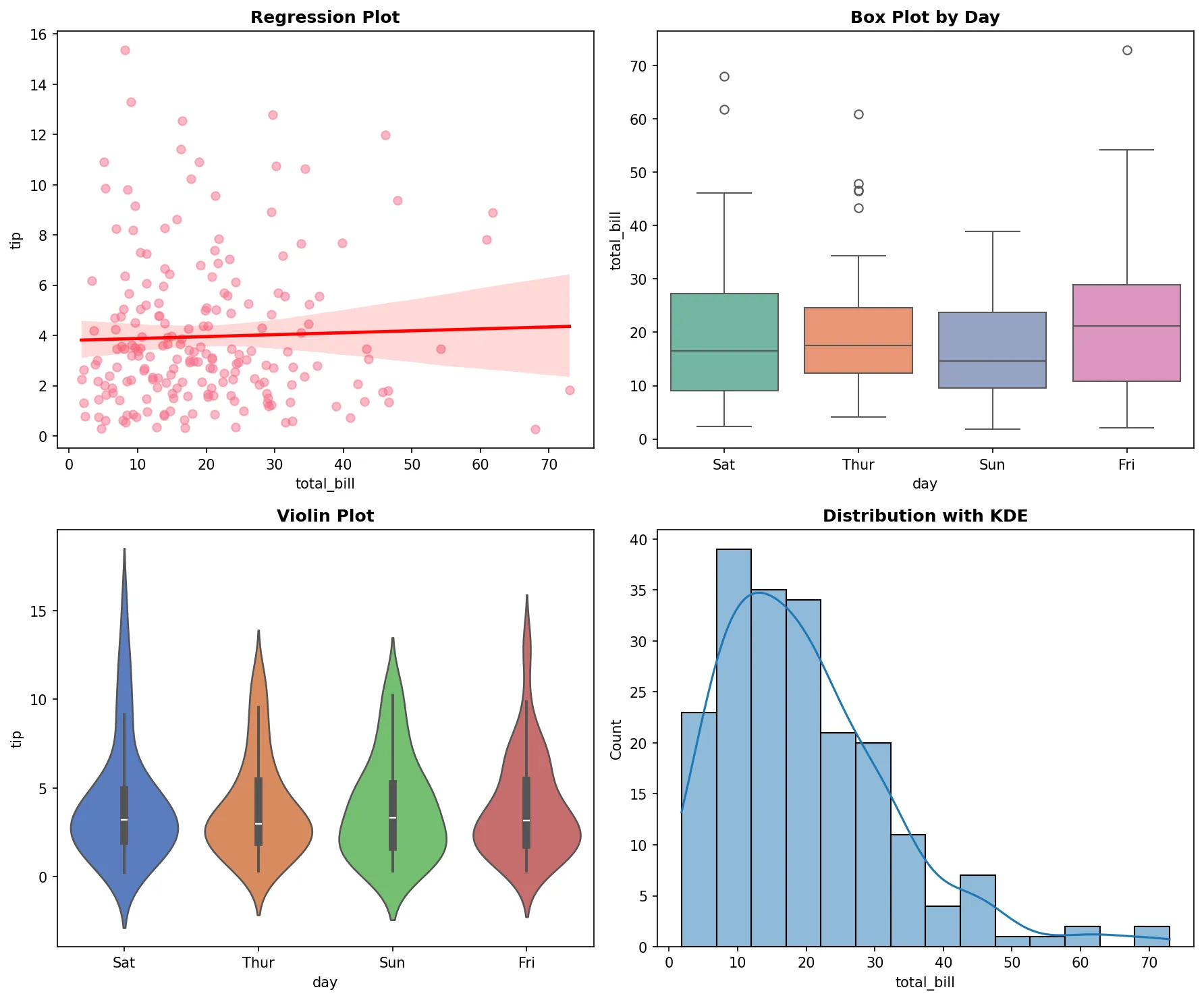

seaborn excels at creating beautiful statistical visualizations with automatic styling and color choices.

Advanced seaborn Features

Reference:

• sns.pairplot(df) - Pairwise relationships
• sns.jointplot(x='col1', y='col2', data=df) - Joint distribution
• sns.violinplot(data=df, x='col1', y='col2') - Violin plot
• sns.stripplot(data=df, x='col1', y='col2') - Strip plot
• sns.catplot(kind='box', data=df, x='col1', y='col2') - Categorical plot

Example:

# Advanced seaborn visualizations
fig, axes = plt.subplots(2, 2, figsize=(15, 12))

# Pair plot (shows all pairwise relationships)
# Note: This creates its own figure, so we'll use a subset
sample_data = tips.sample(50)
sns.pairplot(sample_data, hue='time', height=3)

# Joint plot (scatter + histograms)
sns.jointplot(data=tips, x='total_bill', y='tip', kind='hex')

# Violin plot (shows distribution shape)
sns.violinplot(data=tips, x='day', y='tip', ax=axes[0, 0])
axes[0, 0].set_title('Tip Distribution by Day (Violin Plot)')

# Strip plot (shows individual points)
sns.stripplot(data=tips, x='day', y='tip', hue='time', ax=axes[0, 1])
axes[0, 1].set_title('Individual Tips by Day and Time')

plt.tight_layout()
plt.show()

Density Plots and Distribution Visualization

Density plots show the shape of your data distribution - they’re like histograms but smoother, revealing patterns that might be hidden in discrete bins.

Density plots (also called KDE - Kernel Density Estimation) provide a smooth representation of data distribution.

Reference:

• df.plot.density() - Create density plot
• sns.histplot(data=df, x='col', kde=True) - Histogram with density overlay
• sns.kdeplot(data=df, x='col') - Pure density plot
• sns.distplot(data=df, x='col') - Combined histogram and density

Example:

# Create sample data with different distributions
np.random.seed(42)
normal_data = np.random.normal(0, 1, 1000)
bimodal_data = np.concatenate([
    np.random.normal(-2, 0.5, 500),
    np.random.normal(2, 0.5, 500)
])

# Density plots
fig, axes = plt.subplots(2, 2, figsize=(12, 10))

# pandas density plot
pd.Series(normal_data).plot.density(ax=axes[0, 0], title='Normal Distribution')
axes[0, 0].grid(True, alpha=0.3)

# seaborn density plot
sns.kdeplot(data=normal_data, ax=axes[0, 1], title='Normal Distribution (seaborn)')
axes[0, 1].grid(True, alpha=0.3)

# Bimodal distribution
sns.kdeplot(data=bimodal_data, ax=axes[1, 0], title='Bimodal Distribution')
axes[1, 0].grid(True, alpha=0.3)

# Combined histogram and density
sns.histplot(data=normal_data, kde=True, ax=axes[1, 1], title='Histogram + Density')
axes[1, 1].grid(True, alpha=0.3)

plt.tight_layout()
plt.show()

LIVE DEMO!

Modern Visualization Libraries

The Python visualization ecosystem is constantly evolving. While matplotlib and seaborn are the workhorses, modern libraries offer exciting new approaches.

vega-altair: Grammar of Graphics with Vega-Lite

altair uses a declarative approach where you describe the data mapping rather than specifying drawing commands. It implements the grammar of graphics through Vega-Lite.

altair implements the Vega-Lite grammar of graphics, providing a declarative approach to creating statistical visualizations. It’s designed for interactive web-based visualizations and supports multiple output formats.

Chart Creation and Mark Types

altair uses a simple pattern: create a chart, specify the mark type, and encode your data.

Reference:

• alt.Chart(data) - Create chart from data
• alt.Chart(data).mark_circle() - Scatter plot
• alt.Chart(data).mark_bar() - Bar chart
• alt.Chart(data).mark_line() - Line plot
• alt.Chart(data).mark_area() - Area chart
• alt.Chart(data).mark_rect() - Heatmap/rectangles
• alt.Chart(data).mark_point() - Point plot

Example:

import altair as alt
import pandas as pd

# Sample data
data = pd.DataFrame({
    'x': [1, 2, 3, 4, 5],
    'y': [2, 4, 1, 5, 3],
    'category': ['A', 'B', 'A', 'C', 'B']
})

# Scatter plot - shows relationships between variables
scatter = alt.Chart(data).mark_circle().encode(x='x', y='y')
scatter.show()

# Bar chart - compares values across categories
bar = alt.Chart(data).mark_bar().encode(x='category', y='y')
bar.show()

# Line chart - shows trends over ordered data
line = alt.Chart(data).mark_line().encode(x='x', y='y')
line.show()

# Combined view using altair's concatenation
combined = alt.hconcat(scatter, bar, line)
combined.show()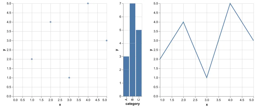

Combined altair charts: scatter plot (left), bar chart (middle), line plot (right)

Data Encoding

The .encode() method maps data columns to visual properties using type annotations.

Reference:

• x='column:Q' - Quantitative (continuous) data
• y='column:O' - Ordinal (discrete) data
• color='column:N' - Nominal (categorical) data
• size='column:Q' - Size encoding
• shape='column:N' - Shape encoding
• tooltip=['col1', 'col2'] - Hover information

Example:

# Enhanced scatter plot with encoding
chart = alt.Chart(data).mark_circle().encode(
    x='x:Q',                    # Quantitative x-axis
    y='y:Q',                    # Quantitative y-axis
    color='category:N',         # Color by category
    size='y:Q',                 # Size by y-value
    tooltip=['x', 'y', 'category']  # Hover info
)

chart.show()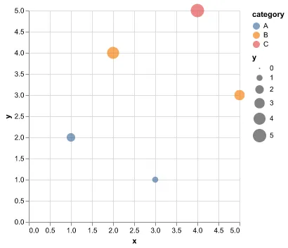

Enhanced scatter plot with color encoding by category and size encoding by y-value

Interactive Features

altair provides built-in interactivity through the .interactive() method, enabling zoom, pan, and selection.

Reference:

• .interactive() - Enable zoom/pan
• .add_selection() - Add selection tools
• .transform_filter() - Filter data dynamically
• alt.selection_interval() - Rectangle selection
• alt.selection_single() - Point selection

Example:

# Interactive scatter plot
interactive_chart = alt.Chart(data).mark_circle().encode(
    x='x:Q',
    y='y:Q',
    color='category:N',
    tooltip=['x', 'y', 'category']
).interactive()

interactive_chart.show()

Advanced altair Features

Faceting and Layering

altair supports faceting (small multiples) and layering multiple mark types.

Reference:

• .facet('column:N') - Create small multiples
• alt.layer() - Combine multiple mark types
• .properties(width=300, height=200) - Set chart dimensions

Example:

# Faceted chart
faceted = alt.Chart(data).mark_circle().encode(
    x='x:Q',
    y='y:Q',
    color='category:N'
).facet('category:N', columns=2)

# Layered chart
base = alt.Chart(data).encode(x='x:Q', y='y:Q')
layered = alt.layer(
    base.mark_circle(color='lightblue'),
    base.mark_line(color='red').transform_regression('x', 'y')
)

Statistical Transformations

altair includes built-in statistical transformations.

Reference:

• .transform_regression('x', 'y') - Add regression line
• .transform_aggregate() - Group and aggregate data
• .transform_filter() - Filter data based on selections

Example:

# Chart with regression line
regression = alt.Chart(data).mark_circle().encode(
    x='x:Q',
    y='y:Q'
) + alt.Chart(data).mark_line(color='red').transform_regression(
    'x', 'y'
).encode(x='x:Q', y='y:Q')

Export Formats

altair supports multiple output formats for different use cases.

Reference:

• chart.save('plot.png') - Static bitmap (PNG)
• chart.save('plot.svg') - Static vector (SVG)
• chart.save('plot.html') - Interactive HTML
• chart.save('plot.json') - Vega-Lite JSON specification

Example:

# Export to different formats
chart.save('scatter.png')      # Static bitmap
chart.save('scatter.svg')      # Static vector
chart.save('interactive.html') # Interactive HTML

Other Modern Tools: plotnine, Bokeh, and Plotly

plotnine: ggplot2 for Python

plotnine brings R’s ggplot2 syntax to Python, perfect for those familiar with R.

Key Features:

• Grammar of graphics approach
• Layered plotting syntax
• Familiar to R users
• Statistical transformations

Reference:

• ggplot(data, aes(x='col1', y='col2')) - Base plot
• + geom_point() - Add scatter points
• + geom_smooth() - Add trend line
• + facet_wrap('~column') - Create facets
• + theme_minimal() - Apply themes

Example:

# Simple scatter plot with ggplot2 syntax
(ggplot(tips, aes(x='total_bill', y='tip', color='time'))
 + geom_point()
 + theme_minimal())

Bokeh: Interactive Web Visualizations

Bokeh creates interactive web-based visualizations with rich interactivity.

Key Features:

• High-performance interactive plots
• Web-based output
• Custom JavaScript callbacks
• Server applications

Reference:

• figure() - Create plot figure
• .circle(), .line(), .bar() - Add glyphs
• HoverTool() - Add hover information
• output_notebook() - Display in Jupyter

Plotly: Interactive Dashboards

Plotly excels at creating interactive dashboards and web applications.

Key Features:

• Easy-to-use API
• Rich interactivity
• Dashboard capabilities
• Multiple chart types

Reference:

• px.scatter(), px.line(), px.bar() - Express functions
• go.Figure() - Graph objects
• make_subplots() - Multiple plots
• .show() - Display plot

Example:

import plotly.express as px

# Simple interactive scatter plot
fig = px.scatter(tips, x='total_bill', y='tip', color='time',
                 title="Interactive Scatter Plot")
fig.show()

Tool Selection Guide

When to use each tool:

• matplotlib: Custom plots, publication quality, fine control
• seaborn: Statistical plots, beautiful defaults, relationship analysis
• pandas: Quick exploration, basic charts
• altair: Interactive plots, grammar of graphics, web-ready
• plotnine: R users, layered approach, statistical plots
• Bokeh: High-performance web visualizations, custom interactions
• Plotly: Dashboards, web applications, easy interactivity

Tool	Best For	Learning Curve	Interactivity	Output Formats	Grammar
matplotlib	Custom plots, publication quality	High	None	PNG/SVG/PDF	Imperative
seaborn	Statistical plots, beautiful defaults	Low	None	PNG/SVG/PDF	Imperative
pandas	Quick exploration, basic charts	Very Low	None	PNG/SVG/PDF	Imperative
altair	Interactive plots, grammar of graphics	Medium	Built-in	PNG/SVG/HTML/JSON	Declarative
plotnine	R users, layered approach	Medium	None	PNG/SVG/PDF	Declarative
bokeh	Interactive web visualizations	High	High	HTML/JS	Imperative
plotly	Dashboards, web applications	Medium	High	HTML/JS	Declarative

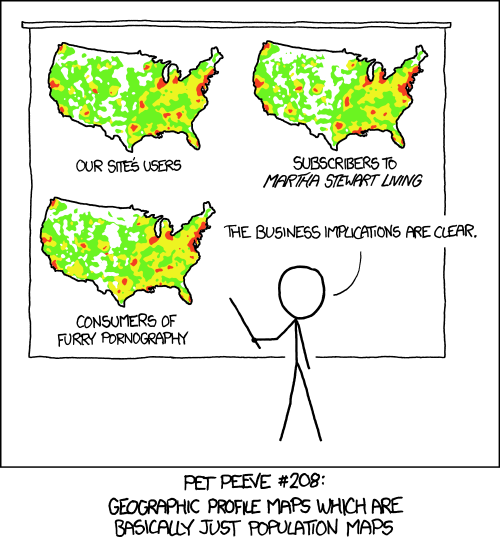
“Every single map of the United States looks the same because it’s just a population density map.” - A reminder that your visualization should show meaningful patterns, not just expected distributions.

LIVE DEMO!