08: Data Wrangling

See Bonus for advanced topics:

• Advanced groupby operations with custom functions
• Hierarchical grouping and MultiIndex operations
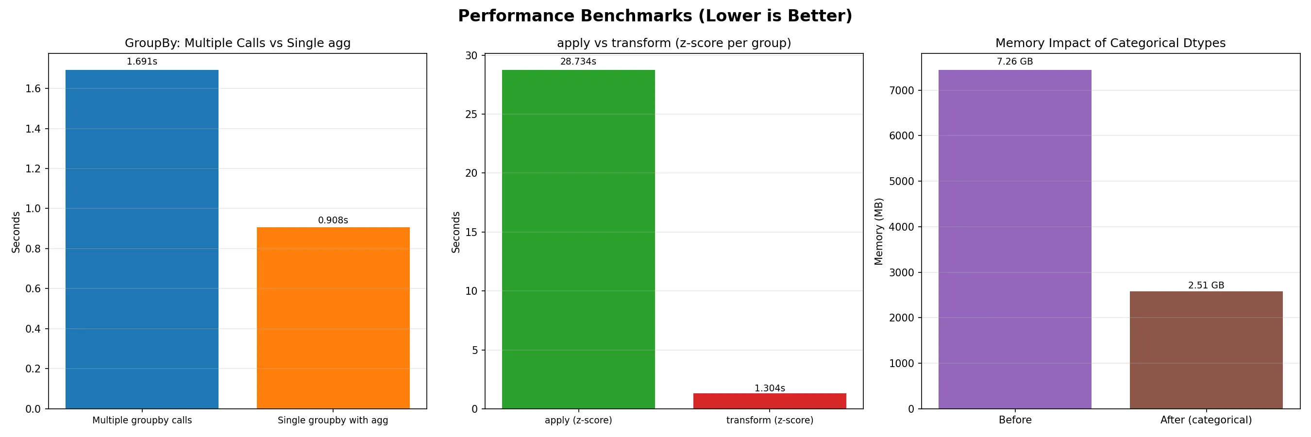
• Performance optimization for large datasets
• Custom aggregation functions and transformations
• Advanced pivot table operations

Outline

• groupby split-apply-combine essentials
• pivot tables and crosstab basics
• remote workflows: ssh, screen, tmux
• performance-minded patterns beginners should know

Fun fact: The term “aggregation” comes from the Latin “aggregare” meaning “to add to a flock.” In data science, we’re literally gathering scattered data points into meaningful groups - turning a flock of individual observations into organized insights.

Data aggregation is the process of summarizing and grouping data to extract meaningful insights. This lecture covers the essential tools for data aggregation: groupby operations, pivot tables, and remote computing for handling large datasets.

The Split-Apply-Combine Paradigm

Reality check: GroupBy operations are the bread and butter of data analysis. Master this concept and you’ll be able to answer almost any “what if we group by…” question that comes your way.

The split-apply-combine paradigm is the foundation of data aggregation. You split data into groups, apply a function to each group, and combine the results.

Visual Guide - GroupBy Operations:

BEFORE GROUPBY                    AFTER GROUPBY
┌─────────┬─────────┬─────────┐   ┌─────────┬─────────┐
│ Category│ Value   │ Other   │   │ Category│ Mean    │
├─────────┼─────────┼─────────┤   ├─────────┼─────────┤
│ A       │ 10      │ X       │   │ A       │ 10.0    │
│ A       │ 15      │ Y       │   │ B       │ 25.0    │
│ B       │ 20      │ Z       │   └─────────┴─────────┘
│ B       │ 25      │ W       │
│ A       │ 5       │ V       │
│ B       │ 30      │ U       │
└─────────┴─────────┴─────────┘

Visual Guide - Split-Apply-Combine:

ORIGINAL DATA                    SPLIT BY CATEGORY
┌─────────┬─────────┬─────────┐   ┌─────────┬─────────┐
│ Category│ Value   │ Other   │   │ Group A │ Group B │
├─────────┼─────────┼─────────┤   ├─────────┼─────────┤
│ A       │ 10      │ X       │   │ A, 10   │ B, 20   │
│ A       │ 15      │ Y       │   │ A, 15   │ B, 25   │
│ B       │ 20      │ Z       │   │ A, 5    │ B, 30   │
│ B       │ 25      │ W       │   └─────────┴─────────┘
│ A       │ 5       │ V       │
│ B       │ 30      │ U       │
└─────────┴─────────┴─────────┘

APPLY FUNCTION (e.g., mean)      COMBINE RESULTS
┌─────────┬─────────┐            ┌─────────┬─────────┐
│ Group A │ Group B │            │ Category│ Mean    │
├─────────┼─────────┤            ├─────────┼─────────┤
│ mean(10,│ mean(20,│            │ A       │ 10.0    │
│ 15, 5)  │ 25, 30)│            │ B       │ 25.0    │
│ = 10.0  │ = 25.0 │            └─────────┴─────────┘
└─────────┴─────────┘

Basic GroupBy Operations

Reference:

• df.groupby('column') - Group by single column
• df.groupby(['col1', 'col2']) - Group by multiple columns
• grouped.mean() - Calculate mean for each group
• grouped.sum() - Calculate sum for each group
• grouped.count() - Count non-null values
• grouped.size() - Count all values (including nulls)
• grouped.agg(['mean', 'sum', 'count']) - Multiple aggregations

Example:

import pandas as pd
import numpy as np

# Create sample data
df = pd.DataFrame({
    'Department': ['Sales', 'Sales', 'Engineering', 'Engineering'],
    'Employee': ['Alice', 'Bob', 'Charlie', 'Diana'],
    'Salary': [50000, 55000, 80000, 85000],
    'Experience': [2, 3, 5, 7]
})

# Basic groupby operations
print("Group by Department:")
print(df.groupby('Department')['Salary'].mean())

print("\nMultiple aggregations:")
print(df.groupby('Department').agg({
    'Salary': ['mean', 'sum'],
    'Experience': 'mean'
}))

Advanced GroupBy Operations

Transform Operations

Transform operations apply a function to each group and return a result with the same shape as the original data.

Reference:

• grouped.transform('mean') - Apply mean to each group
• grouped.transform('std') - Apply standard deviation to each group
• grouped.transform(lambda x: x - x.mean()) - Custom transform function
• grouped.transform(['mean', 'std']) - Multiple transforms

Example:

# Transform: Add group means as new column
df['Salary_Mean'] = df.groupby('Department')['Salary'].transform('mean')
df['Salary_Std'] = df.groupby('Department')['Salary'].transform('std')
df['Salary_Normalized'] = df.groupby('Department')['Salary'].transform(lambda x: (x - x.mean()) / x.std())

print("Data with group statistics:")
print(df[['Department', 'Employee', 'Salary', 'Salary_Mean', 'Salary_Std', 'Salary_Normalized']])

Filter Operations

Filter operations remove entire groups based on a condition.

Reference:

• grouped.filter(lambda x: len(x) > n) - Keep groups with more than n rows
• grouped.filter(lambda x: x['col'].sum() > threshold) - Keep groups meeting condition
• grouped.filter(lambda x: x['col'].mean() > threshold) - Filter by group statistics

Example:

# Filter: Keep only departments with more than 1 employee
filtered = df.groupby('Department').filter(lambda x: len(x) > 1)
print("Departments with multiple employees:")
print(filtered)

# Filter: Keep only departments with average salary > 60000
high_salary_depts = df.groupby('Department').filter(lambda x: x['Salary'].mean() > 60000)
print("\nHigh-salary departments:")
print(high_salary_depts)

Apply Operations

Apply operations let you use custom functions on each group.

Reference:

• grouped.apply(func) - Apply custom function to each group
• grouped.apply(lambda x: x.sort_values('col')) - Sort each group
• grouped.apply(lambda x: x.nlargest(2, 'col')) - Get top 2 from each group
• grouped.apply(func, include_groups=False) - Exclude grouping columns from function (pandas 2.2+)

Important: FutureWarning for include_groups Parameter

Starting in pandas 2.2, when using .apply() on a GroupBy object, pandas will include the grouping columns in the DataFrame passed to your function. This is a change from previous behavior where grouping columns were excluded. To maintain the old behavior (where grouping columns are excluded), you should explicitly set include_groups=False.

What’s happening:

• Old behavior (pandas < 2.2): When you call df.groupby('Department').apply(func), the function receives only the non-grouping columns
• New behavior (pandas 2.2+): By default, the function receives all columns including the grouping columns
• Future behavior: include_groups=False will become the default, but you should explicitly set it now to avoid warnings

Why this matters:

• If your function expects only non-grouping columns, you’ll get unexpected behavior
• The warning helps you prepare for future pandas versions
• Setting include_groups=False explicitly makes your code future-proof

Example:

# Apply: Custom function for salary statistics
def salary_stats(group):
    # With include_groups=False, 'group' contains only non-grouping columns
    # Without it, 'group' also contains 'Department' column
    return pd.Series({
        'count': len(group),
        'mean': group['Salary'].mean(),
        'std': group['Salary'].std(),
        'range': group['Salary'].max() - group['Salary'].min()
    })

print("Custom statistics by department:")
# Explicitly set include_groups=False to avoid FutureWarning
print(df.groupby('Department').apply(salary_stats, include_groups=False))

# Apply: Get top earners in each department
top_earners = df.groupby('Department').apply(
    lambda x: x.nlargest(1, 'Salary'),
    include_groups=False
)
print("\nTop earners per department:")
print(top_earners)

LIVE DEMO!

Hierarchical Grouping

Reference:

• df.groupby(['level1', 'level2']) - Multi-level grouping
• grouped.unstack() - Convert to wide format
• grouped.stack() - Convert to long format
• grouped.swaplevel(0, 1) - Swap grouping levels

Example:

# Create hierarchical data
hierarchical_df = pd.DataFrame({
    'Region': ['North', 'North', 'South', 'South', 'North', 'South'],
    'Department': ['Sales', 'Engineering', 'Sales', 'Engineering', 'Marketing', 'Marketing'],
    'Revenue': [100000, 150000, 120000, 180000, 80000, 90000],
    'Employees': [5, 8, 6, 10, 4, 5]
})

# Hierarchical grouping
hierarchical_grouped = hierarchical_df.groupby(['Region', 'Department']).sum()
print("Hierarchical grouping:")
print(hierarchical_grouped)

# Unstack to wide format
wide_format = hierarchical_grouped.unstack()
print("\nWide format:")
print(wide_format)

Pivot Tables and Cross-Tabulations

Think of pivot tables as the data analyst’s Swiss Army knife - they can reshape, summarize, and analyze data in ways that would take dozens of lines of code to accomplish manually.

Pivot tables are powerful tools for summarizing and analyzing data across multiple dimensions.

Visual Guide - Pivot Table Transformation:

LONG FORMAT (Original)              WIDE FORMAT (Pivoted)
┌─────────┬─────────┬─────────┐     ┌─────────┬─────────┬─────────┐
│ Product │ Region  │ Sales   │     │ Product │ North   │ South   │
├─────────┼─────────┼─────────┤     ├─────────┼─────────┼─────────┤
│ A       │ North   │ 1000    │     │ A       │ 1000    │ 1500    │
│ A       │ South   │ 1500    │     │ B       │ 2000    │ 1200    │
│ B       │ North   │ 2000    │     └─────────┴─────────┴─────────┘
│ B       │ South   │ 1200    │
└─────────┴─────────┴─────────┘

Basic Pivot Tables

Reference:

• pd.pivot_table(df, values='col', index='row', columns='col') - Basic pivot
• pd.pivot_table(df, aggfunc='mean') - Specify aggregation function
• pd.pivot_table(df, fill_value=0) - Fill missing values
• pd.pivot_table(df, margins=True) - Add totals
• pd.crosstab(index, columns) - Cross-tabulation

Example:

# Create sample sales data
sales_data = pd.DataFrame({
    'Product': ['A', 'A', 'B', 'B', 'C', 'C'],
    'Region': ['North', 'South', 'North', 'South', 'North', 'South'],
    'Sales': [1000, 1500, 2000, 1200, 800, 900]
})

# Basic pivot table
pivot = pd.pivot_table(sales_data,
                    values='Sales',
                    index='Product',
                    columns='Region',
                    aggfunc='sum')
print("Sales by Product and Region:")
print(pivot)

# Pivot with multiple aggregations
pivot_multi = pd.pivot_table(sales_data,
                            values='Sales',
                            index='Product',
                            columns='Region',
                            aggfunc=['sum', 'mean'])
print("\nMultiple aggregations:")
print(pivot_multi)

Advanced Pivot Operations

Reference:

• pivot_table(..., margins=True, margins_name='Total') - Add totals
• pivot_table(..., fill_value=0) - Fill missing values
• pivot_table(..., dropna=False) - Keep missing combinations
• pivot_table(..., observed=True) - Include all category combinations

Example:

# Advanced pivot with totals and missing value handling
advanced_pivot = pd.pivot_table(sales_data,
                               values='Sales',
                               index='Product',
                               columns='Region',
                               aggfunc='sum',
                               margins=True,
                               margins_name='Total',
                               fill_value=0)
print("Advanced pivot with totals:")
print(advanced_pivot)

# Cross-tabulation
crosstab = pd.crosstab(sales_data['Product'],
                      sales_data['Region'],
                      margins=True)
print("\nCross-tabulation:")
print(crosstab)

LIVE DEMO!

Remote Computing and SSH

When your data is too big for your laptop, it’s time to think about remote computing. SSH is your gateway to powerful remote servers that can handle massive datasets.

Remote computing allows you to leverage powerful servers for data analysis that would be impossible on your local machine.

SSH Fundamentals

Reference:

• ssh username@hostname - Connect to remote server
• ssh -p port username@hostname - Connect on specific port
• ssh-keygen -t rsa - Generate SSH key pair
• ssh-copy-id username@hostname - Copy public key to server
• scp file username@hostname:path - Copy file to server
• scp username@hostname:file path - Copy file from server

Example:

# Generate SSH key pair
ssh-keygen -t rsa -b 4096 -C "your_email@example.com"

# Copy public key to server
ssh-copy-id username@server.com

# Connect to server
ssh username@server.com

# Copy files to server
scp data.csv username@server.com:~/data/

# Copy files from server
scp username@server.com:~/results/analysis.ipynb ./

Remote Data Analysis

Reference:

# Start Jupyter notebook on remote server
jupyter notebook --ip=0.0.0.0 --port=8888 --no-browser

# Forward port to local machine
ssh -L 8888:localhost:8888 username@server.com

# Access Jupyter at http://localhost:8888
# As if it were running on your local machine

Example:

# Remote data analysis workflow
import pandas as pd
import numpy as np

# Load large dataset on remote server
df = pd.read_csv('/path/to/large_dataset.csv')

# Perform aggregation on remote server
result = df.groupby('category').agg({
    'value': ['mean', 'std', 'count'],
    'other_col': 'sum'
})

# Save results
result.to_csv('aggregated_results.csv')

# Download results to local machine
# scp username@server.com:~/aggregated_results.csv ./

screen and tmux for Persistent Sessions

Screen lets you detach and reattach long-running jobs; tmux is a more modern, scriptable alternative. Use whichever your server offers.

Screen quickstart:

# Create a named screen session
screen -S analysis

# Detach (Ctrl+a d) and list sessions
screen -ls

# Reattach later
screen -r analysis

# Kill session from inside
exit

tmux quickstart:

Reference:

# tmux commands
tmux new-session -s analysis
tmux list-sessions
tmux attach-session -t analysis
tmux kill-session -t analysis

# Inside tmux
Ctrl+b d  # Detach from session
Ctrl+b c  # Create new window
Ctrl+b n  # Next window
Ctrl+b p  # Previous window

Example:

# Start persistent analysis session
tmux new-session -s data_analysis

# Inside tmux, start your analysis
conda activate datasci_217
jupyter notebook --ip=0.0.0.0 --port=8888

# Detach from session (Ctrl+b, then d)
# Session continues running on server

# Reattach later
tmux attach-session -t data_analysis

Performance Optimization

When working with large datasets, every millisecond counts. Understanding performance optimization can mean the difference between a 5-minute analysis and a 5-hour analysis.

Efficient GroupBy Operations

Reference:

# Optimize groupby operations
def efficient_groupby(df, group_cols, agg_cols):
    """Efficient groupby with optimized operations"""

    # Use categorical data types for grouping columns
    for col in group_cols:
        if df[col].dtype == 'object':
            df[col] = df[col].astype('category')

    # Use specific aggregation functions
    result = df.groupby(group_cols)[agg_cols].agg({
        'numeric_col': ['mean', 'sum'],
        'other_col': 'count'
    })

    return result

# Memory-efficient operations
## Note: chunking manually for larger-than-memory data should be a last resort.
## It is usually faster to rely on package-provided options.
def memory_efficient_analysis(df):
    """Analyze large dataset with chunking"""

    # Process in chunks
    chunk_size = 10000
    results = []

    for chunk in pd.read_csv('large_file.csv', chunksize=chunk_size):
        # Process chunk
        chunk_result = chunk.groupby('category').sum()
        results.append(chunk_result)

    # Combine results
    final_result = pd.concat(results).groupby(level=0).sum()
    return final_result

Parallel Processing (optional)

Reference:

from multiprocessing import Pool
import pandas as pd

def process_chunk(chunk):
    """Process a single chunk of data"""
    return chunk.groupby('category').sum()

def parallel_groupby(df, n_processes=4):
    """Parallel groupby processing"""

    # Split data into chunks
    chunk_size = len(df) // n_processes
    chunks = [df.iloc[i:i+chunk_size] for i in range(0, len(df), chunk_size)]

    # Process in parallel
    with Pool(n_processes) as pool:
        results = pool.map(process_chunk, chunks)

    # Combine results
    return pd.concat(results).groupby(level=0).sum()

LIVE DEMO!