09: Visualization

See Bonus for advanced topics:

• Advanced time series decomposition and seasonal analysis
• Time series forecasting with ARIMA and exponential smoothing
• Period arithmetic and fiscal year handling
• High-frequency data analysis and tick data
• Custom frequency classes and time zone complexities

Fun fact: Time series analysis is like being a detective for data - you’re looking for patterns, trends, and clues that reveal the story of how things change over time. It’s the difference between knowing what happened and understanding why it happened.

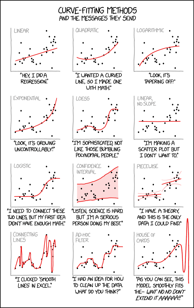
“Cauchy-Lorentz: ‘Something alarmingly mathematical is happening, and you should probably stop.’” - A reminder that not every pattern in time series data is meaningful, and overfitting is always lurking.

Time series analysis is the art of understanding temporal patterns in data. This lecture covers the essential tools for time series analysis: datetime handling, resampling and frequency conversion, rolling window operations, and time series indexing and selection.

Pro tip: Time series analysis is 90% datetime wrangling, 5% actual analysis, and 5% swearing at timezone conversions. Master these datetime tools and you’ll be ahead of 90% of data scientists.

Learning Objectives:

• Master datetime data types and parsing
• Perform time series indexing and selection
• Use resampling and frequency conversion
• Apply rolling window operations
• Understand exponentially weighted functions
• Handle basic time zone operations

Understanding Time Series Data

Reality check: Time series data is everywhere in health and medical research - patient vital signs, clinical trial measurements, disease surveillance, environmental monitoring. Understanding how to work with temporal data is essential for any data scientist in the life sciences.

Time series data is characterized by observations collected over time, where the order and timing of observations matter. Unlike cross-sectional data, time series data has a natural temporal structure that we can exploit for analysis.

Types of Time Series

“Time series data comes in many flavors - some are as regular as a Swiss watch, others as unpredictable as a toddler’s nap schedule. The key is knowing which one you’re dealing with!”

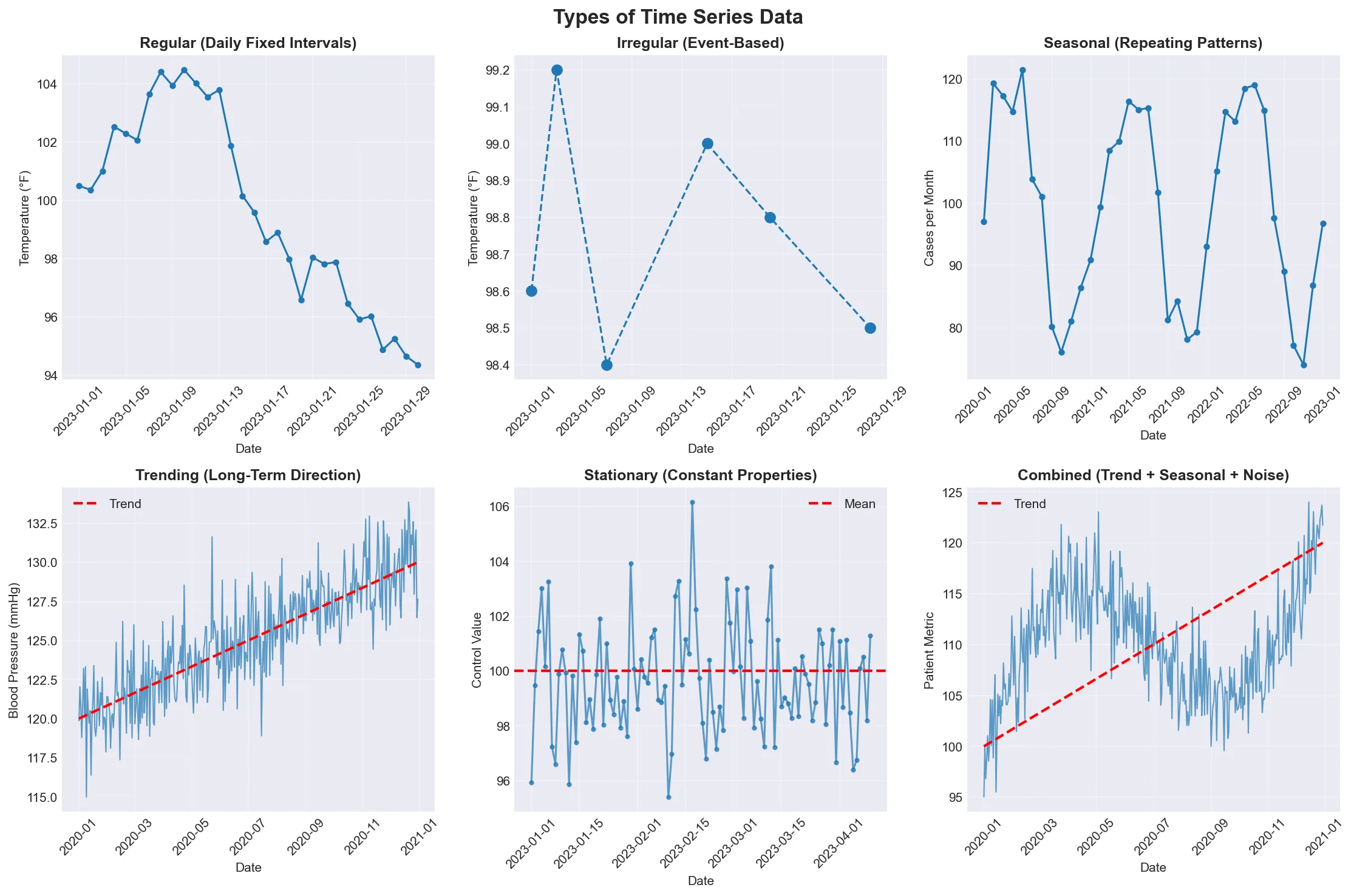
Visual guide showing the different types of time series data. Notice how regular series tick along like clockwork, while irregular series jump around like a medical appointment schedule.

Type	Description	Example
Regular	Fixed intervals (daily, hourly, monthly)	Daily patient temperature readings
Irregular	Variable intervals (event-based)	Clinical visit dates
Seasonal	Patterns repeat over time	Monthly flu case counts
Trending	Long-term direction	Long-term blood pressure trends
Stationary	Statistical properties don’t change	Laboratory control measurements
Combined	Multiple components (trend + seasonal + noise)	Real-world medical data with all patterns

Date and Time Data Types

Think of datetime objects as the Swiss Army knife of temporal data - they can represent any moment in time with precision down to microseconds, and pandas makes them incredibly powerful for analysis.

Python datetime Module

The Python standard library provides datetime for working with dates and times. Understanding these basics is essential before moving to pandas. Think of it as learning to walk before you can run - except in this case, walking is parsing dates and running is resampling multi-site clinical trial data.

Reference:

Function	Description
datetime.now()	Current date and time
datetime(year, month, day)	Create specific date
datetime.strptime(string, format)	Parse string to datetime
datetime.strftime(format)	Format datetime to string
timedelta(days=1)	Time differences

Example:

from datetime import datetime, timedelta

# Current time
now = datetime.now()
print(f"Current time: {now}")

# Specific date (patient birth date)
birthday = datetime(1990, 5, 15)
print(f"Birth date: {birthday}")

# String parsing (lab result timestamp)
date_str = "2023-12-25 14:30:00"
parsed_date = datetime.strptime(date_str, "%Y-%m-%d %H:%M:%S")
print(f"Parsed date: {parsed_date}")

# String formatting
formatted = parsed_date.strftime("%B %d, %Y at %I:%M %p")
print(f"Formatted: {formatted}")

# Time differences (age calculation)
time_diff = now - birthday
print(f"Age in days: {time_diff.days}")

pandas DatetimeIndex

pandas provides powerful datetime functionality through DatetimeIndex, which is optimized for time series operations.

Reference:

Function	Description
pd.to_datetime()	Convert to datetime
pd.date_range()	Create date range
pd.DatetimeIndex()	Create datetime index
df.set_index('date')	Set datetime index
df.index	Access datetime index

Example:

# Convert to datetime (lab test dates)
date_strings = ['2023-01-01', '2023-01-02', '2023-01-03']
dates = pd.to_datetime(date_strings)
print("Converted dates:")
print(dates)

# Create date range (daily patient monitoring)
date_range = pd.date_range('2023-01-01', periods=10, freq='D')
print("\nDate range:")
print(date_range)

# Create DataFrame with datetime index (vital signs)
df = pd.DataFrame({
    'heart_rate': np.random.randint(60, 100, 10),
    'blood_pressure': np.random.randint(90, 140, 10)
}, index=date_range)
print("\nDataFrame with datetime index:")
print(df.head())

Important Note: When setting a datetime column as the index for DataFrames with multiple rows per date (e.g., multiple patients measured on the same date), pandas may have trouble with date range selection using .loc.

Prerequisites: First, convert your date column to datetime and set it as the index:

df['date'] = pd.to_datetime(df['date'])  # Convert to datetime
df = df.set_index('date')  # Set as index

The Problem: If your DataFrame has multiple patients with measurements on the same date, the index might look like [2023-01-01, 2023-01-02, 2023-01-01, 2023-01-03, ...] - notice dates aren’t in order. Pandas can’t reliably slice date ranges on non-monotonic indexes.

The Solution: Sort the index: df = df.sort_index(). This makes the index monotonic (non-decreasing), so all rows with the same date are grouped together: [2023-01-01, 2023-01-01, 2023-01-02, 2023-01-03, ...]. Now date range selection like df.loc['2023-01':'2023-03'] works correctly.

Date Range Generation

pandas provides flexible date range generation for creating regular time series. Want every Monday? Got it. Business days only? No problem. Last Friday of each month? Absolutely. Third Wednesday? Why not! pandas can generate pretty much any date pattern you can imagine - and some you probably can’t.

Reference:

Function	Frequency Code	Description
pd.date_range(start, end, freq='D')	'D'	Daily (calendar)
pd.bdate_range(start, end)	'B'	Business days only
pd.date_range(freq='W-MON')	'W-MON'	Weekly on Monday
pd.date_range(freq='MS')	'MS'	Month start
pd.date_range(freq='QS')	'QS'	Quarter start
pd.date_range(freq='H')	'H'	Hourly

Note: Both ‘H’ and ‘h’ work for hourly frequency, but ‘H’ is the canonical form.

Example:

# Different date range types for clinical data
print("Daily range (vital signs):")
daily = pd.date_range('2023-01-01', '2023-01-10', freq='D')
print(daily)

print("\nBusiness days only (clinic visits):")
business = pd.bdate_range('2023-01-01', '2023-01-10')
print(business)

print("\nWeekly range (Mondays - weekly checkups):")
weekly = pd.date_range('2023-01-01', '2023-03-01', freq='W-MON')
print(weekly)

print("\nMonthly range (monthly lab tests):")
monthly = pd.date_range('2023-01-01', '2023-12-01', freq='MS')
print(monthly)

Frequency Inference

You can infer the frequency of a time series and convert between frequencies.

Reference:

Function	Description
pd.infer_freq(ts.index)	Infer frequency from time series
ts.asfreq(freq)	Convert to specific frequency
ts.resample(freq).asfreq()	Resample and convert frequency

Example:

# Create time series with inferred frequency
dates = pd.date_range('2023-01-01', periods=100, freq='D')
ts = pd.Series(np.random.randn(100), index=dates)

# Infer frequency
freq = pd.infer_freq(ts.index)
print(f"Inferred frequency: {freq}")

# Convert to different frequency (daily to weekly)
ts_weekly = ts.asfreq('W')
print(f"Weekly frequency: {pd.infer_freq(ts_weekly.index)}")

Shifting and Lagging

Shifting allows you to create lagged or leading versions of your time series, essential for analyzing changes over time.

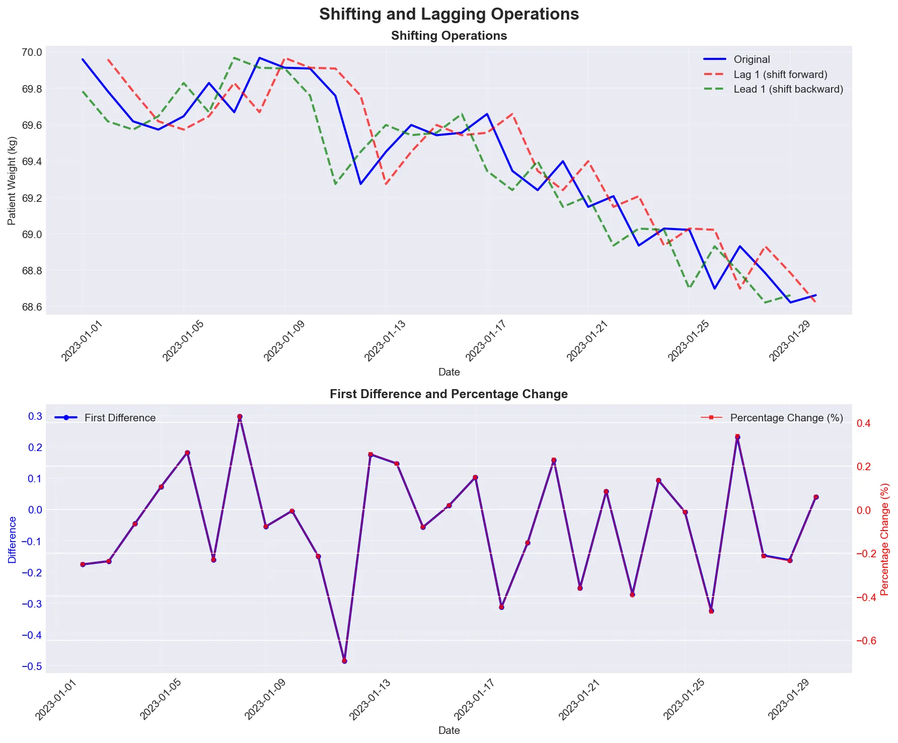
Visual demonstration of shifting operations showing lag (looking back), lead (looking ahead), and differences (day-to-day changes).

Reference:

Function	Description
ts.shift(1)	Shift by 1 period (lag)
ts.shift(-1)	Shift by -1 period (lead)
ts.diff()	First difference
ts.pct_change()	Percentage change
ts.shift(1, freq='D')	Shift by 1 day (with timestamp)

Example:

# Create sample time series (patient weight measurements)
dates = pd.date_range('2023-01-01', periods=10, freq='D')
ts = pd.Series([70.5, 70.8, 70.2, 71.0, 70.9, 71.2, 71.5, 71.3, 71.8, 71.6], index=dates)

# Shifting operations
ts['lag_1'] = ts.shift(1)  # Previous day
ts['lead_1'] = ts.shift(-1)  # Next day
ts['diff'] = ts.diff()  # First difference (day-to-day change)
ts['pct_change'] = ts.pct_change()  # Percentage change

print("Time series with shifts:")
print(ts[['lag_1', 'diff', 'pct_change']].head())

LIVE DEMO!

Time Series Indexing and Selection

Basic Time Series Selection

pandas provides intuitive ways to select data from time series using string-based indexing. You can write “2023” and pandas knows you mean “all of 2023”.

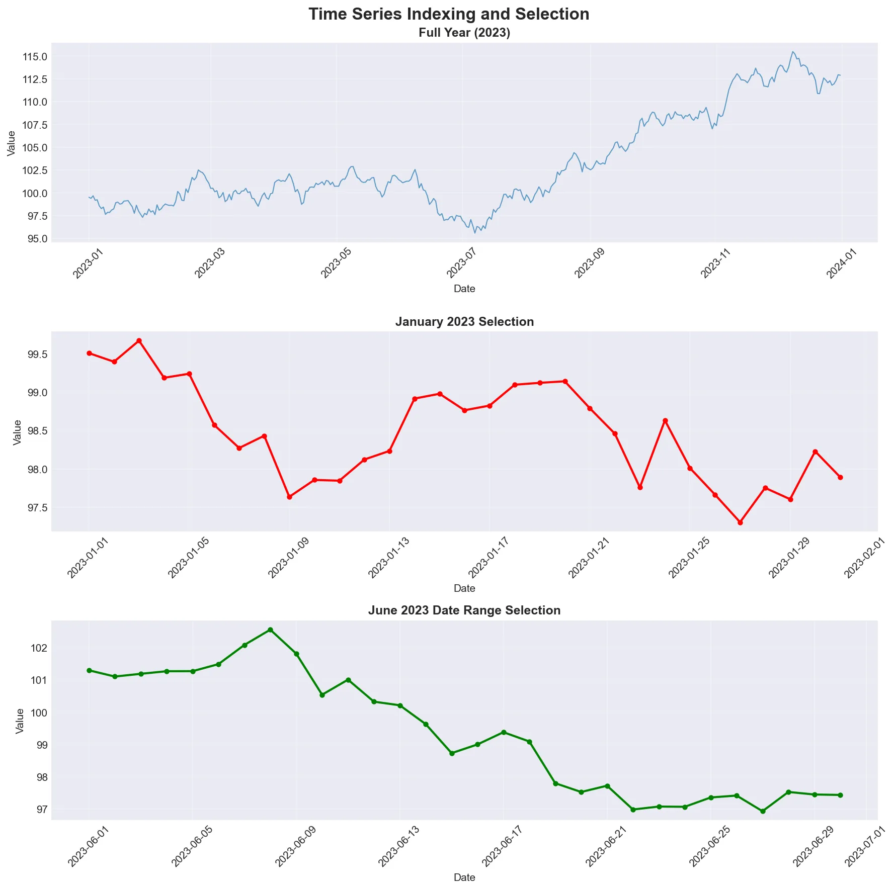
Examples of time-based selection showing how to slice data by year, month, or date range. Notice how pandas interprets string dates like a human would.

Reference:

Operation	Description
ts['2023-01-01']	Select specific date
ts['2023-01-01':'2023-01-31']	Select date range
ts['2023']	Select entire year
ts['2023-01']	Select specific month
ts.loc['2023-01-01']	Label-based selection
ts.iloc[0:10]	Position-based selection

Example:

# Create sample time series (year of patient data)
dates = pd.date_range('2023-01-01', periods=365, freq='D')
values = np.cumsum(np.random.randn(365)) + 100
ts = pd.Series(values, index=dates)

# Select specific date
print("January 1, 2023:")
print(ts['2023-01-01'])

# Select date range
print("\nJanuary 2023:")
print(ts['2023-01-01':'2023-01-31'].head())

# Select entire year
print("\n2023 data shape:")
print(ts['2023'].shape)

# Select specific month
print("\nJanuary 2023:")
print(ts['2023-01'].head())

Advanced Time Series Selection

For time series with time components, you can select based on time of day. This is useful for selecting data from business hours or specific times of day.

Reference:

Function	Description
ts.between_time('09:00', '17:00')	Select time range
ts.at_time('12:00')	Select specific time
ts.loc[:start_date + pd.Timedelta(days=9)]	First 10 days
ts.loc[end_date - pd.Timedelta(days=9):]	Last 10 days
ts.truncate(before='2023-06-01')	Truncate before date (requires sorted index)
ts.truncate(after='2023-06-30')	Truncate after date (requires sorted index)

Example:

# Create hourly time series (ICU monitoring)
hourly_dates = pd.date_range('2023-01-01', periods=24*7, freq='H')
hourly_values = np.random.randn(24*7) + 100
ts_hourly = pd.Series(hourly_values, index=hourly_dates)

# Select business hours (9 AM to 5 PM)
business_hours = ts_hourly.between_time('09:00', '17:00')
print("Business hours data:")
print(business_hours.head())

# Select specific time (noon readings)
noon_data = ts_hourly.at_time('12:00')
print("\nNoon data:")
print(noon_data.head())

# Select first and last periods using .loc
print("\nFirst 3 days:")
first_3_days = ts_hourly.loc[:ts_hourly.index.min() + pd.Timedelta(days=2)]
print(first_3_days.head())

print("\nLast 3 days:")
last_3_days = ts_hourly.loc[ts_hourly.index.max() - pd.Timedelta(days=2):]
print(last_3_days.head())

Resampling and Frequency Conversion

Resampling is like changing the lens on your camera - you can zoom in to see more detail (higher frequency) or zoom out to see the big picture (lower frequency).

Resampling converts time series from one frequency to another. Downsampling aggregates higher frequency data to lower frequency (e.g., daily to monthly). Upsampling converts lower frequency to higher frequency (e.g., monthly to daily), often introducing missing values.

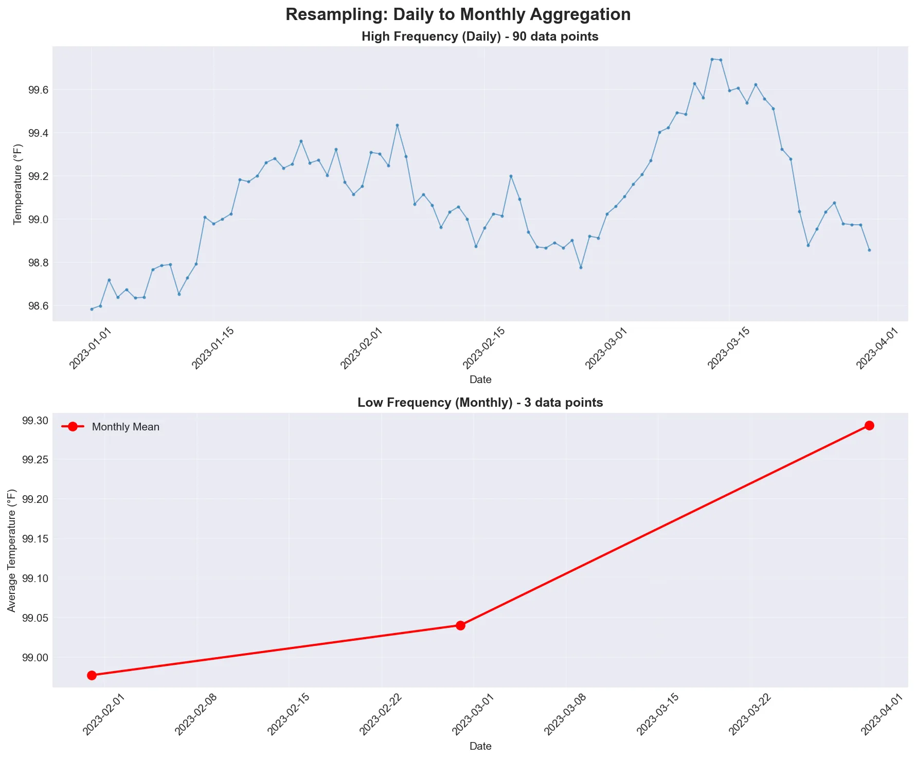
Visual comparison showing daily data (high frequency, many points) being resampled to monthly data (low frequency, fewer points). Notice how the monthly view smooths out daily fluctuations.

Basic Resampling

The resample() method is the workhorse for frequency conversion, similar to groupby() but for time intervals.

Reference:

Frequency Code	Description
ts.resample('D')	Daily resampling
ts.resample('W')	Weekly resampling
ts.resample('ME')	Monthly resampling (Month End)
ts.resample('Q')	Quarterly resampling
ts.resample('A')	Annual resampling
ts.resample('H')	Hourly resampling

Example:

# Create daily time series (patient vital signs)
daily_dates = pd.date_range('2023-01-01', periods=30, freq='D')
daily_values = np.cumsum(np.random.randn(30)) + 100
ts_daily = pd.Series(daily_values, index=daily_dates)

# Resample to different frequencies
print("Original daily data shape:", ts_daily.shape)

# Weekly resampling (average weekly values)
weekly = ts_daily.resample('W').mean()
print("Weekly resampled shape:", weekly.shape)
print("Weekly data:")
print(weekly.head())

# Monthly resampling (average monthly values)
monthly = ts_daily.resample('ME').mean()  # 'ME' = Month End
print("\nMonthly resampled shape:", monthly.shape)
print("Monthly data:")
print(monthly.head())

Resampling with Different Aggregations

You can apply various aggregation functions when resampling, just like with groupby(). The syntax is the same, but instead of grouping by categories, you’re grouping by time intervals.

Important Note: When resampling DataFrames that contain non-numeric columns (like patient IDs or category labels), you’ll get an error if you try to aggregate them with numeric functions like mean(). Use df.select_dtypes(include=[np.number]) to select only numeric columns before resampling, or specify which columns to aggregate in .agg().

Reference:

Function	Description
ts.resample('D').mean()	Mean aggregation
ts.resample('D').sum()	Sum aggregation
ts.resample('D').max()	Maximum aggregation
ts.resample('D').min()	Minimum aggregation
ts.resample('D').std()	Standard deviation
ts.resample('D').agg(['mean', 'std', 'min', 'max'])	Multiple aggregations

Example:

# Create sample data with multiple columns (patient metrics)
df = pd.DataFrame({
    'temperature': np.random.normal(98.6, 0.5, 365),
    'heart_rate': np.random.randint(60, 100, 365)
}, index=pd.date_range('2023-01-01', periods=365, freq='D'))

# Different resampling methods
print("Daily to weekly resampling:")
weekly_stats = df.resample('W').agg({
    'temperature': ['mean', 'std', 'min', 'max'],
    'heart_rate': 'mean'
})
print(weekly_stats.head())

# Custom resampling function
def custom_agg(series):
    return pd.Series({
        'mean': series.mean(),
        'std': series.std(),
        'range': series.max() - series.min(),
        'count': len(series)
    })

print("\nCustom aggregation:")
custom_stats = df['temperature'].resample('ME').apply(custom_agg)
print(custom_stats.head())

LIVE DEMO!

Rolling Window Operations

Rolling window functions compute statistics over a fixed-size window that moves through the time series. This is useful for smoothing noisy data and identifying trends.

Basic Rolling Operations

The rolling() method creates a rolling window object that can be used with various aggregation functions.

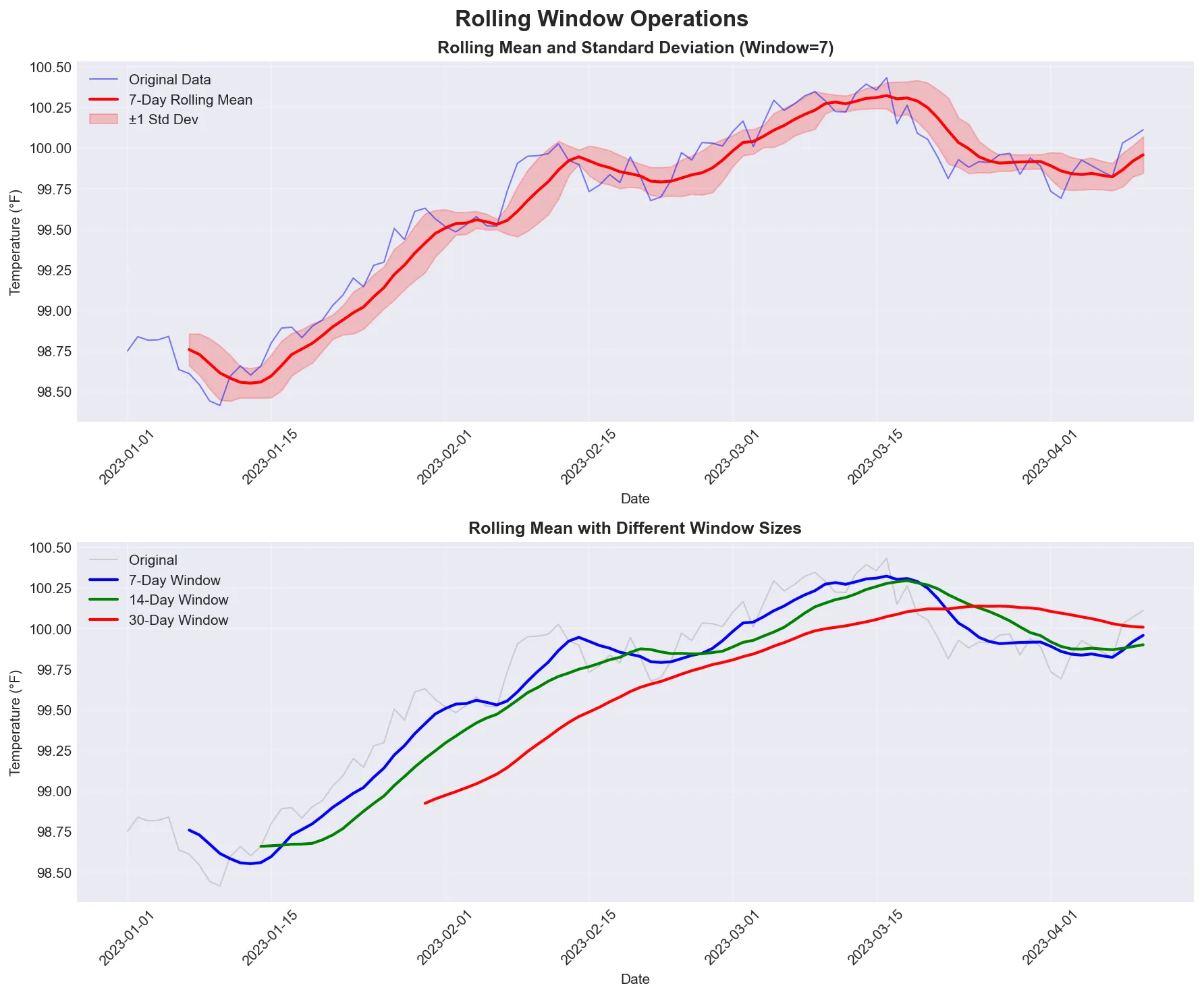
Demonstration of rolling window operations showing how a 7-day window smooths out daily fluctuations while preserving the underlying trend. The shaded area shows the standard deviation - wider means more variability, narrower means more consistent.

Reference:

Function	Description
ts.rolling(window=5)	5-period rolling window
ts.rolling(window=5).mean()	Rolling mean
ts.rolling(window=5).std()	Rolling standard deviation
ts.rolling(window=5).sum()	Rolling sum
ts.rolling(window=5).min()	Rolling minimum
ts.rolling(window=5).max()	Rolling maximum

Example:

# Create sample time series (patient temperature over time)
dates = pd.date_range('2023-01-01', periods=100, freq='D')
values = 98.6 + np.cumsum(np.random.randn(100) * 0.1)  # Temperature with drift
ts = pd.Series(values, index=dates)

# Rolling statistics (7-day rolling window)
ts['rolling_mean'] = ts.rolling(window=7).mean()
ts['rolling_std'] = ts.rolling(window=7).std()
ts['rolling_min'] = ts.rolling(window=7).min()
ts['rolling_max'] = ts.rolling(window=7).max()

print("Time series with rolling statistics:")
print(ts[['rolling_mean', 'rolling_std']].head(10))

Advanced Rolling Operations

Rolling windows can be centered, have minimum periods, and use custom functions. Centered windows look both backward and forward from each point. Minimum periods allow calculations even before you have a full window.

Reference:

Function	Description
ts.rolling(window=5, center=True)	Centered rolling window
ts.rolling(window=5, min_periods=3)	Minimum periods required
ts.rolling(window=5).quantile(0.5)	Rolling median
ts.rolling(window=5).apply(custom_func)	Custom rolling function
ts.expanding()	Expanding window (from start to current)
ts.ewm(span=5)	Exponentially weighted moving average

Example:

# Advanced rolling operations
ts['centered_mean'] = ts.rolling(window=7, center=True).mean()
ts['expanding_mean'] = ts.expanding().mean()  # Mean from start to current
ts['ewm_mean'] = ts.ewm(span=7).mean()  # Exponentially weighted

# Custom rolling function
def rolling_range(series):
    return series.max() - series.min()

ts['rolling_range'] = ts.rolling(window=7).apply(rolling_range)

print("Advanced rolling statistics:")
print(ts[['centered_mean', 'expanding_mean', 'ewm_mean']].head(10))

Exponentially Weighted Functions

Exponentially weighted functions give more weight to recent observations, making them more responsive to recent changes.

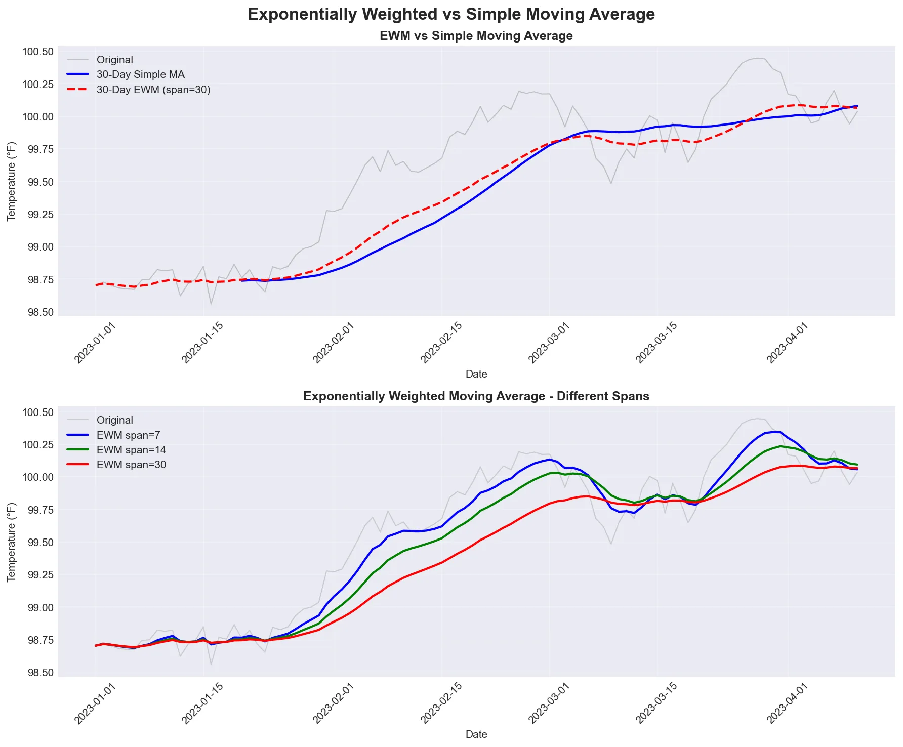
Comparison of exponentially weighted moving average (EWM) with simple moving average. Notice how EWM responds faster to recent changes.

Reference:

Function	Description
ts.ewm(span=5).mean()	Exponentially weighted moving average
ts.ewm(alpha=0.3).mean()	EWM with alpha parameter
ts.ewm(halflife=2).mean()	EWM with half-life
ts.ewm(span=5).std()	Exponentially weighted standard deviation

Example:

# Create sample time series (patient blood pressure)
dates = pd.date_range('2023-01-01', periods=50, freq='D')
ts = pd.Series(np.cumsum(np.random.randn(50)) + 120, index=dates)

# Exponentially weighted functions
ts['ewm_mean'] = ts.ewm(span=5).mean()
ts['ewm_std'] = ts.ewm(span=5).std()
ts['ewm_alpha'] = ts.ewm(alpha=0.3).mean()

print("Time series with EWM functions:")
print(ts[['ewm_mean', 'ewm_std']].head(10))

“You can’t fall off the bell curve if there’s no bell curve.” - A reminder that time series forecasting, especially during unprecedented events, carries significant uncertainty. Always be honest about prediction intervals.

Time Zone Handling

“I find it hard to believe that a time zone can be a real thing.” - A relatable sentiment when dealing with time zone conversions.

Basic Time Zone Operations

pandas provides time zone localization and conversion for timezone-aware datetime objects.

Best Practice: When working with time zones, use UTC (Coordinated Universal Time) as your base timezone. UTC has no daylight saving time, avoiding ambiguity issues. Store data in UTC, and convert to local timezones only when needed for display or analysis.

Reference:

Function	Description
ts.index.tz_localize('UTC')	Add timezone to naive datetime
ts.index.tz_convert('US/Eastern')	Convert timezone
pd.Timestamp.now(tz='UTC')	Current time in timezone
pd.date_range(..., tz='UTC')	Create timezone-aware date range

Example:

# Create timezone-aware datetime (clinical trial data)
utc_time = pd.Timestamp.now(tz='UTC')
print(f"UTC time: {utc_time}")

# Convert to different timezone (US Eastern)
eastern_time = utc_time.tz_convert('US/Eastern')
print(f"Eastern time: {eastern_time}")

# Create timezone-aware DataFrame
df_tz = pd.DataFrame({
    'value': np.random.randn(3)
}, index=pd.date_range('2023-01-01', periods=3, freq='D'))

# Localize to UTC
df_tz.index = df_tz.index.tz_localize('UTC')
print("\nUTC DataFrame:")
print(df_tz)

# Convert to Eastern time
df_tz.index = df_tz.index.tz_convert('US/Eastern')
print("\nEastern DataFrame:")
print(df_tz)

Time Series Visualization

Visualization is essential for understanding time series data. A good plot can reveal patterns, trends, and anomalies that summary statistics miss.

Basic Time Series Plots

Creating effective time series visualizations helps identify patterns, trends, and anomalies. The most common visualization is a simple line plot showing values over time.

Reference:

Function	Description
ts.plot()	Basic line plot of time series
ts.plot(figsize=(12, 6))	Plot with custom figure size
ts.plot(title='Title')	Plot with title
ts.plot(style='-', marker='o')	Plot with custom style and markers
ax = ts.plot()	Get axes for further customization

Example:

import matplotlib.pyplot as plt

# Create sample time series (patient temperature over year)
dates = pd.date_range('2023-01-01', periods=365, freq='D')
values = 98.6 + 2 * np.sin(2 * np.pi * np.arange(365) / 365.25) + np.random.randn(365) * 0.5
ts = pd.Series(values, index=dates)

# Basic time series plot
ts.plot(figsize=(12, 6), title='Patient Temperature Over Time',
        xlabel='Date', ylabel='Temperature (°F)')
plt.grid(True, alpha=0.3)
plt.tight_layout()
plt.show()

# Plot with rolling mean overlay
fig, ax = plt.subplots(figsize=(12, 6))
ts.plot(ax=ax, alpha=0.5, label='Daily', color='gray')
ts.rolling(window=30).mean().plot(ax=ax, linewidth=2, label='30-Day Rolling Mean', color='blue')
ax.set_title('Patient Temperature with Rolling Mean', fontsize=14, fontweight='bold')
ax.set_xlabel('Date')
ax.set_ylabel('Temperature (°F)')
ax.legend()
ax.grid(True, alpha=0.3)
plt.tight_layout()
plt.show()

![media/viz_temp.png]

![media/viz_temp_rolling.png]

Visualizing Time Series Components

Real-world time series data often contains multiple components: trend, seasonality, and noise. Visualizing these components separately helps understand the underlying patterns.

Example:

# Create time series with trend, seasonal, and noise components
dates = pd.date_range('2023-01-01', periods=365, freq='D')
trend = np.linspace(100, 120, 365)  # Long-term trend
seasonal = 10 * np.sin(2 * np.pi * np.arange(365) / 365.25)  # Seasonal pattern
noise = np.random.randn(365) * 3  # Random noise
combined = trend + seasonal + noise
ts = pd.Series(combined, index=dates)

# Visualize components separately
fig, axes = plt.subplots(4, 1, figsize=(12, 12), sharex=True)

# Original combined series
ts.plot(ax=axes[0], title='Original (Trend + Seasonal + Noise)', color='black')
axes[0].set_ylabel('Value')

# Trend component
pd.Series(trend, index=dates).plot(ax=axes[1], title='Trend Component', color='blue')
axes[1].set_ylabel('Value')

# Seasonal component
pd.Series(seasonal, index=dates).plot(ax=axes[2], title='Seasonal Component', color='green')
axes[2].set_ylabel('Value')

# Noise component
pd.Series(noise, index=dates).plot(ax=axes[3], title='Noise Component', color='red', alpha=0.7)
axes[3].set_ylabel('Value')
axes[3].set_xlabel('Date')

for ax in axes:
    ax.grid(True, alpha=0.3)

plt.tight_layout()
plt.show()

![media/viz_components.png]

Note: For advanced seasonal decomposition techniques (like STL decomposition), see Bonus.

LIVE DEMO!